13 Neutrino Astronomy

Diffuse flux of Astrophysical Neutrinos

The first detection of high-energy neutrinos of cosmic origin in 2013 by the IceCube Neutrino Observatory opened a new window to the non-thermal processes in our universe. The first strong evidence for a cosmic neutrino component came from a search using data from May 2010 to April 2012 [35], where two shower-like events from interactions within the detector with energies above 1 PeV were discovered. A follow-up search for events starting in the detector with more than 30 TeV deposited energy that utilized the same dataset identified 25 additional high-energy events. The spectrum and zenith angle distribution of the events was incompatible with the hypothesis of an atmospheric origin at > $4\sigma$. IceCube has since collected independent evidence for an astrophysical neutrino signal by analyzing different event signatures.

Starting Events

Neutrino interactions are identified in IceCube by searching for an interaction vertex within the instrumented volume. This search is sensitive to both shower-like and track-like events. Since the main background for this search is comprised of muons from CR air showers, the rejection strategy is to identify Cherenkov photons from a track entering the detector. For that, the outer parts of the instrumented volume are assigned to a “veto” region. An event is rejected if a certain number of Cherekov photons are found in this veto region at earlier times than the photons produced at the interaction vertex. The energy threshold for this analysis is about $E_\nu \sim 30$ TeV.

Through-going muons

Muons produced in CC neutrino interactions far outside the detector can still reach the instrumented volume to produce track-like events. Even at 1 TeV a muon can penetrate several kilometers of ice before it stops and decays. This allows observation of high-energy neutrino interactions from a much larger volume than the instrumented one, thereby substantially increasing the effective area of the detector.

The spectral fit

The results of a combined analysis fits the neutrino flux to a power-law between 27 TeV and 2 PeV consistent with an unbroken power law with a best-fit spectral index given by:

\[E^2\Phi(E) = 2.06^{+0.35}_{-0.26} \times 10^{-8} \left(\frac{E}{100\;\mathrm{TeV}}\right)^{-0.46\pm 0.12}\; \mathrm{GeV\;s}^{-1}\;\mathrm{sr}^{-1}\mathrm{ cm}^{-2}.\]

However using only the high energy through-going muons (abouve 200 TeV) yields a preferred spectral index of $-2.13\pm 0.13$

The Search for Point Sources

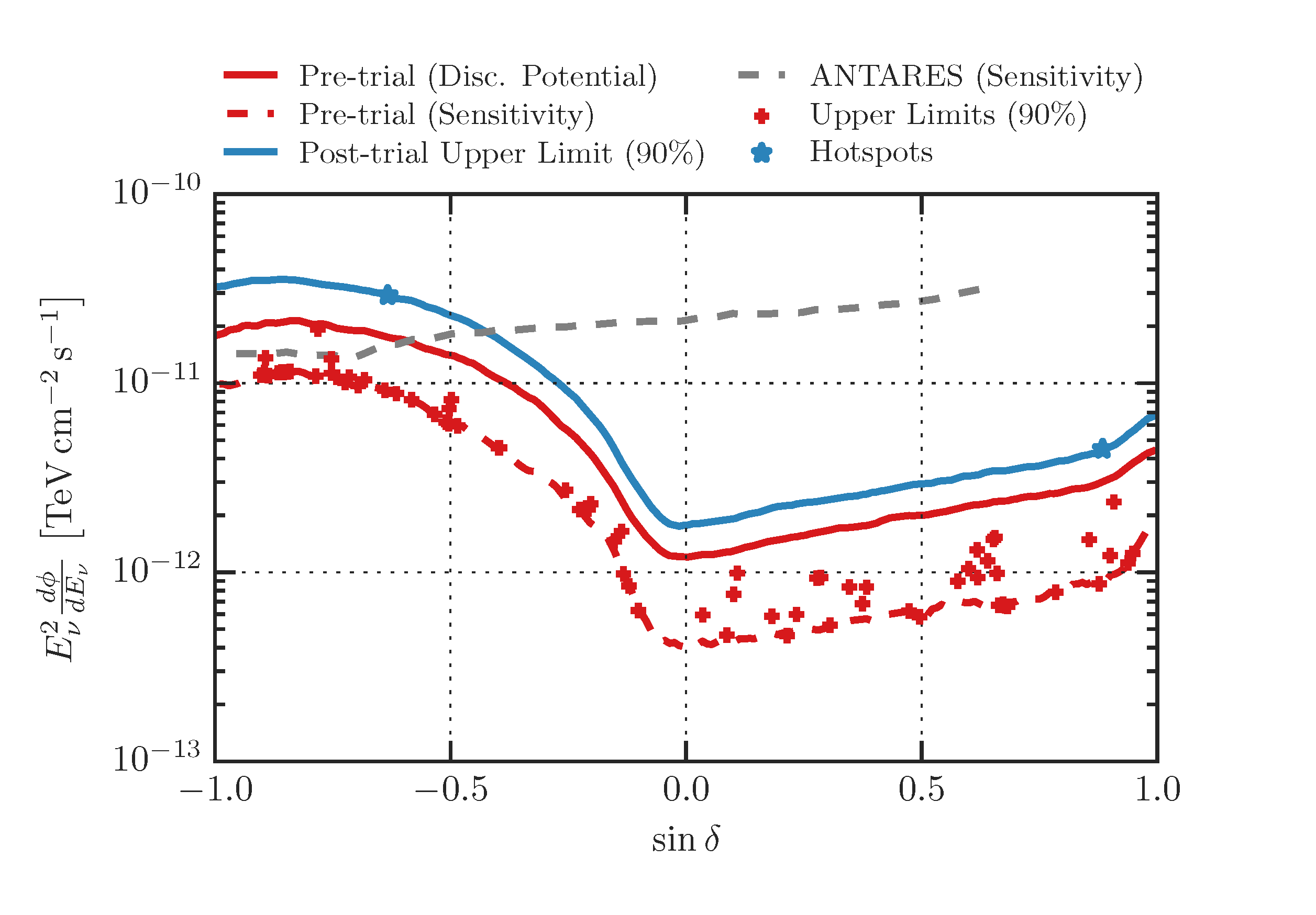
In the case where the cosmic neutrino flux is dominated by bright individual sources, they should be detectable as a local excess of events on the sky with respect to the atmospheric neutrino and diffuse cosmic neutrino background. The sensitivity of a search for such features depends crucially on the precision by which the direction of the neutrinos can be reconstructed from the data, i.e. on the detector angular resolution. No indication for a neutrino point source has been found in the IceCube data so far. The null result of a point-source of neutrinos, can be transformed into an flux upper limit at a given confidence level. This upper limits represents the neutrino flux that we can be certain to exclude, since IceCube did not see a point source.

The Olbers’ Paradox

Altough the most famous formulation of the problem comes from Henrich Olbers (1826), probably it was Kepler in 1610 the first to note that the most obvious observation, the night sky is dark, has very important consequences.

The idea is quite simple, suppose there is a source population with typical luminosity $L$ in ergs/s and a number density of $n$, then the total power emitted per unit area will be:

\[ F = \int L n \frac{dV}{4\pi^2} = \frac{1}{4\pi}\int L n \mathrm{ d}\Omega \mathrm{ d}r\]

Integrating over all distances we can obtain the energy per steradian per second, and assuming the luminosity is independent of distance as well as number density we have that:

\[\frac{\mathrm{ d} F}{\mathrm{ d}\Omega} = \frac{1}{4\pi} L n \int_0^{\infty} \mathrm{ d}r \rightarrow \infty\]

The sky should be bright! The solution of this puzzle is the fact the Universe is dynamic and time dependent! In other words, if the Universe is expanding the radiation from increasingly distant sources is increasingly less. Also stars seems to have had a cosmological evolution, for example, there are more quasars per unit volume at $z \sim 2$ than now.

Although the Olbers’ paradox is no more a paradox, it represents the problem that arises with neutrino astronomy. Since the extragalactic space is completely transparent for neutrinos, the flux of neutrinos that might arrive at Earth will have a significant contribution from very distant and faint sources. Let’s assume now a source population with typical neutrino luminosity $L\nu(E)$ and with a number density population given by:

\[n(z) = n_0 (1+z)^m\]

where $n_0$ is the local density of the source population, (ie the population close to our epoch $z = 0$). The parameter $m$ describes the source cosmological evolution (ie, when sources to appear in the history of the Universe, and how they evolved). Typical values are $m= 3$ for star–formation–like evolution and $m=0$ for no evolution.

Since the Universe expands and sources move with the Huble flow we are going to use the comoving line of sight distance, defined as (see Lecture 2):

\[D_c(z) = \int_{t}^{t_0} c\mathrm{ d} t = \frac{c}{H_0} \int^z_0 \frac{\mathrm{ d}z^\prime}{E(z^\prime)}\]

where we introduced the function:

\[E(z)\equiv \sqrt{\Omega_M(1+z)^4 + \Omega_r(1+z)^5 + \Omega_k(1+z)^3 +\Omega_\Lambda(1+z)}\]

revisiting the formula of the energy rate of neutrinos per steroradian we have:

\[\frac{\mathrm{ d} F_\nu}{\mathrm{ d}\Omega} = \frac{1}{4\pi} \frac{c}{H_0}\int_0^{\infty} \frac{L_\nu(E_\nu) n_0(1+z)^m}{E(z)} \mathrm{ d}z\]

The expresion above needs an extra correction. We assumed that energy emitted by the source will be the same at the arrival, however energy will be red-shifted according to $E_\nu (1 + z)$ so the formula it’s technically:

\[\frac{\mathrm{ d} F_\nu}{\mathrm{ d}\Omega} = \frac{1}{4\pi} \frac{c}{H_0}\int_0^{\infty} \frac{L_\nu(E_\nu(1+z)) n_0(1+z)^m}{E(z)} \mathrm{ d}z\]

Assuming the luminosity follows a power law with, $L_\nu \propto E^{-\gamma}$, we can rewrite the expression as:

\[\frac{\mathrm{ d} F_\nu}{\mathrm{ d}\Omega} = \xi \frac{c}{H_0} \frac{L_\nu(E_\nu) n_0}{4\pi} \]

where the unit-less parameter $\xi$ is the integral that contains information on the expansion and cosmological evolution of the sources and the spectral index of the sources defined as:

\[\xi = \int_0^{\infty}\frac{(1+z)^{(m - \gamma)}\mathrm{ d} z}{E(z)}\]

Assuming an spectral index of 2, and expressing it as function of the scale factor knowing that:

\[\frac{\mathrm{ d}z}{1+z} = - \frac{\mathrm{ d}a}{a} \rightarrow \mathrm{ d}z = -\frac{\mathrm{ d}a}{a^2}\]

and that $z = \infty \rightarrow a = 0$, $z = 0 \rightarrow a = 1$, we can rewrite the integral as:

\[\xi = \int_0^{1}\frac{a^{-m} \mathrm{ d} a}{E(a)}\]

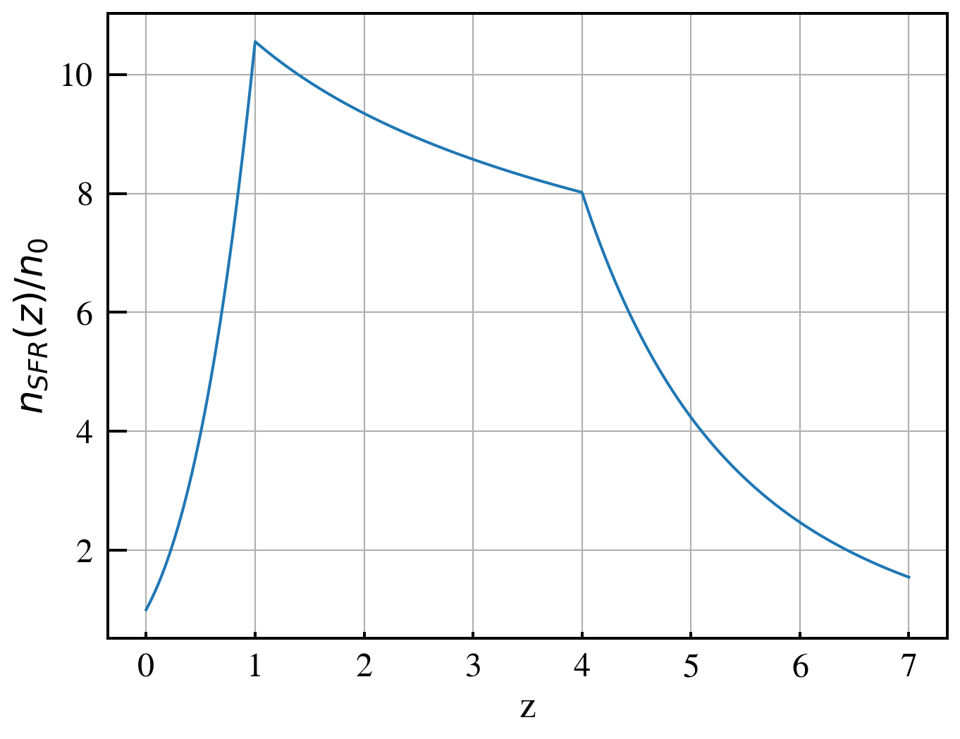
Where it will depend on the cosmic evolution of the sources. Typical star forming rate evolution (SFR) has an evolution of $m = 3.4$ in our local universe $z<1 $ and $m=-0.3$ for $ 1< z< 4$ and $m=-3.5$ elsewhere.

Tutorial I: Calculate the value of $\xi$

We are going to calculate the value of the parameter $\xi$ for different cosmological evolution of the sources. The SFR evolution is given by the following broken power law formula:

import numpy as np
import matplotlib.pylab as plt
plt.rcParams['font.family'] = "STIXGeneral"
plt.rcParams.update({'axes.labelsize': 20})
plt.rcParams.update({'legend.fontsize': 20})
plt.rcParams.update({'figure.figsize': [8, 6]})
plt.rcParams['xtick.labelsize'] = 18
plt.rcParams['ytick.labelsize'] = 18
plt.rcParams['xtick.major.width'] = 1.5
plt.rcParams['xtick.minor.width'] = 1
plt.rcParams['xtick.major.pad'] = 8
plt.rcParams['xtick.direction'] = 'in'
plt.rcParams['ytick.major.size'] = 10
plt.rcParams['ytick.minor.size'] = 5
plt.rcParams['ytick.major.width'] = 1.5
plt.rcParams['ytick.minor.width'] = 1
plt.rcParams['ytick.major.pad'] = 8
plt.rcParams['ytick.direction'] = 'in'
plt.rcParams['legend.frameon'] = False
plt.rcParams['lines.linewidth'] = 1.5
plt.rcParams['axes.linewidth'] = 1.5

def rho(z):
    if z < 1.:
        return (1. + z)**3.4
    elif z >= 1. and z <= 4.:
        return (1+1.)**3.4 * ((1.+z)/(1.+1.))**-0.3
    else:
        return (1.+1.)**3.4*((1.+4.)/(1.+1.))**-0.3*((1.+z)/(1.+4.))**-3.5
    
ax = plt.subplot(111)

z = np.linspace(0, 7, 1000)
vrho = np.vectorize(rho)

ax.plot(z, vrho(z))
ax.set_xlabel("z")
ax.set_ylabel("$n_{SFR}(z)/n_0$")
ax.grid()

from astropy.cosmology import Planck13 as cosmo
from scipy import integrate

def xi(z):
    return cosmo.H0.value/cosmo.H(z).value * rho(z) * (1 + z)**(-2)

integral = integrate.quad(lambda z: xi(z), 0., np.inf)[0]

print(r"$\xi$ = %.2f for an evolution of SFR" %(integral))

integral = integrate.quad(lambda z: cosmo.H0.value/cosmo.H(z).value  * (1 + z)**(-2), 0., 2)[0]

print(r"$\xi$ = %.2f for no cosmological evolution up to redshift z < 2" %(integral))

$\xi$ = 2.39 for an evolution of SFR
$\xi$ = 0.48 for no cosmological evolution up to redshift z < 2

Therefore the parameter $\xi$ varies between $0.5\sim 3$. We can equate this total neutrino flux per steroradian to the flux observed by IceCube (assuming an spectral index of 2):

\[\xi \frac{c}{H_0} \frac{L_\nu(E_\nu) n_0}{4\pi} = E^2 \Phi_\nu \sim 2.06 \times 10^{-8} \frac{\mathrm{ GeV}}{\mathrm{ cm}^2\mathrm{ s\;} \mathrm{ sr}}\]

#I'm going to use units to avoid stupid mistakes
import astropy.units as u
from astropy import constants as const
from IPython.display import display, Markdown

xi = 0.48

icecube_flux = 2.06e-8 * u.GeV/u.cm**2/u.s/u.sr

Ln = icecube_flux * cosmo.H0.to(1/u.s)/const.c.to(u.Mpc/u.s) * 4 * np.pi * u.sr * xi
Ln = Ln.to(u.erg/u.Mpc**3/u.yr)

display(Markdown(r"$n_0 L_\nu \sim$ {0:.1e} {1}".format(Ln.value, Ln.unit.to_string("latex"))))

$n_0 L_\nu \sim$ 1.4e+43 $\mathrm{\frac{erg}{yr\,Mpc^{3}}}$

ie, it reaches the value of:

\[n_0 L_\nu \sim 10^{43} \frac{\mathrm{erg}}{\mathrm{Mpc}^3\mathrm{yr}}\]

note that this is almost independent of the value of $xi$. We can represent this relation in a diagram now called Kowalski’s plot:

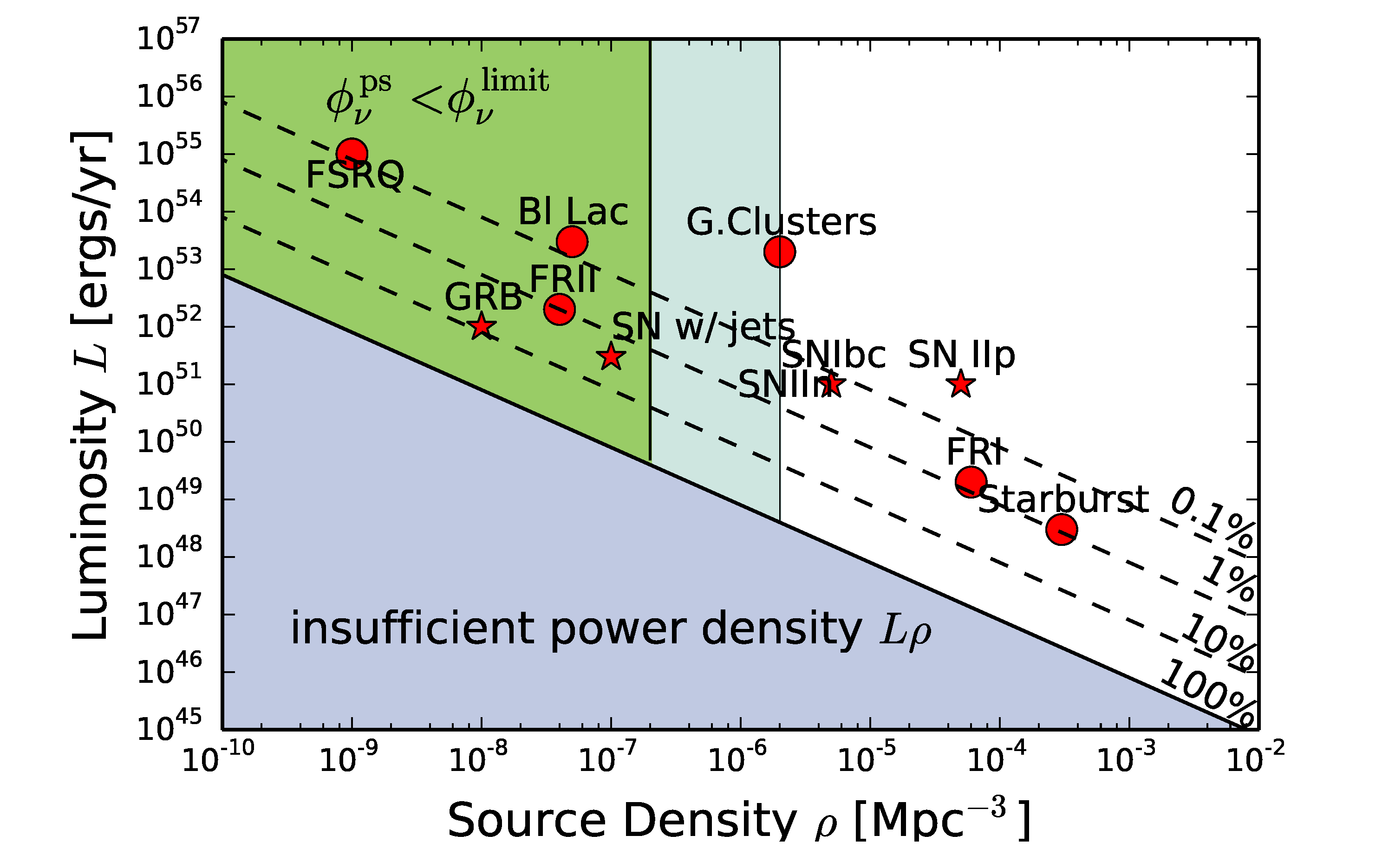
Constrains can also be obtained from the point-source limits. The argument is as follows, if the source population that is responsible of the diffuse astrophysical flux observed in IceCube, is rate (has a low density) then the closest of these sources should have provided a signal in the point-source analysis. Let’s assume that $d$ is the distance to the nearest source for a source population with local density $n_0$ so:

\[n_0 \frac{4}{3} \pi d^3 = 1\]

since there is 1 source in an sphere of radius $d$. We can estimate the closest distance to a source of this population as:

\[ d = \left(\frac{1}{\frac{4}{3}\pi n_0}\right)^{1/3} \propto n_0^{-1/3}\]

and thus the estimated neutrino flux for this single point-source is:

\[E^2 \Phi^{ps}_\nu = \frac{L_\nu}{4\pi d^2} \sim L_\nu n_0^{2/3}\]

A typical value of the neutrino point-source upper limits can be obtained for the Northern sky as:

\[E^2 \Phi^{u.l.}_\nu \leq 2 \times 10^{-9} \mathrm{ GeV} \mathrm{ cm}^{-2}\mathrm{ s}^{-1} \]

so we have the 2 constrains together:

\[n_0^{-1/3} \leq \frac{\Phi^{u.l.}}{10^{43}\frac{\mathrm{erg}}{\mathrm{Mpc}^3\mathrm{yr}}}\]

which leads to the following condition on the local density of sources from the point-source upper limits:

flux_upperlimit = 2e-9 * u.GeV/u.cm**2 / u.s

n0 = np.power(flux_upperlimit/Ln, -3)
n0 = n0.to(u.Mpc**-3)

display(Markdown(r"$n_0 \geq$ {0:.1e} {1}".format(n0.value, n0.unit.to_string("latex_inline"))))

$n_0 \geq$ 2.8e-06 $\mathrm{Mpc^{-3}}$

References

High energy neutrinos in the context of multimessenger astrophysics. J. Becker arXiv:0710.1557v2
Cosmic Neutrinos from the Sources of Galactic and Extragalactic Cosmic Rays. F. Halzen arxiv:0611915