If a source of the light is moving away from an observer, then redshift (z > 0) occurs; if the source moves towards the observer, then blueshift (z < 0) occurs. This is true for all electromagnetic waves and is explained by the Doppler effect. Consequently, this type of redshift is called the Doppler redshift.
Relativistic Redshift
The wavefront moves with velocity \(c\), but at the same time the source moves away with velocity \(v\). Afte a time \(t_s\) the source has receded \(vt\). The crest of the wave emission is at \(\lambda+v t_s=ct_s\). The period in the reference system of the source is given by:
Since \(\Delta x_{o} =0\) (we are just measuring when the crest of the waves arrive), then the time observed \(t_{o}\) in the reference system O is given:
\[t_o = \frac{t_s}{\gamma}.\]
The corresponding observed frequency is \[f_o = \frac{1}{t_o} = \gamma (1-\beta) f_s = \sqrt{\frac{1-\beta}{1+\beta}}\,f_s.\]
In the non-relativistic limit (when \(v \ll c\)) this redshift can be approximated by \(z \simeq \beta = \frac{v}{c}\) corresponding to the classical Doppler effect.
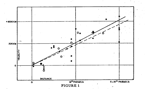
Hubble Expansion
When plotting their redshift (ie speed) as function of distance (measured with the techniques we saw, parallax, etc.) in 1929 Hubble found a correlation between redshift and radial distance from Earth:
\[v = H_0 r, \; H_0 = 72\;\mathrm{ km/s/Mpc}\]
Note that \(H_0\) has only units of time\(^{-1}\) we explicitely write the other dimensions to better understand its meaning.
But Doppler redshift does not depends on distance! So this not a doppler redshift but a Cosmological redshift. In this case the redshift is not due to relative velocities, the photons instead increase in wavelength and redshift because the spacetime through which they are traveling is expanding.
But we said that for midly relativistic objects (and galaxies are moving at midly relativistic speeds) we can approximate \(z \approx \beta\) so we can use \(z\) to estimate distances!:
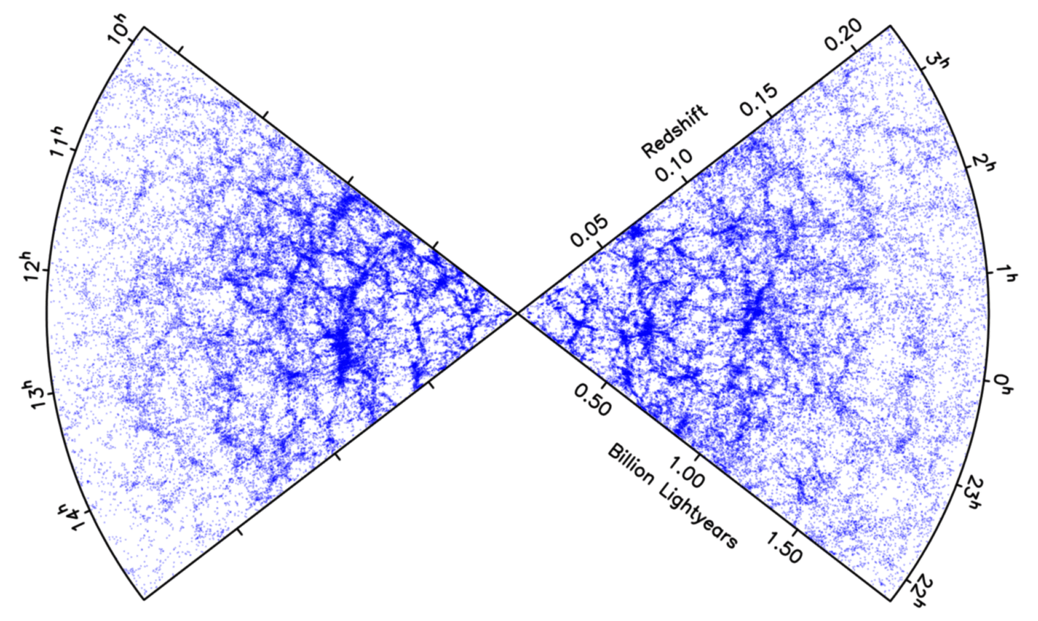
The cosmological principle is the notion that the distribution of matter in the Universe is homogeneous and isotropic when viewed on a large enough scale.
Homogeneity states that the distribution of matter is even in each epoch.
Isotropy states that there are no prefered directions in the distribution of matter in space.
The End of Greatness is an observational scale discovered at roughly 100 Mpc where the lumpiness seen in the large-scale structure of the universe is homogenized and isotropized, this together with the isotropy of the CMB reinforced the idea of the Cosmological Principle.
However, in 2013 a new structure 3 Gpc wide has been discovered, the Hercules–Corona Borealis Great Wall, which puts doubt on the validity of the cosmological principle.
Friedmann–Lemaître-Robertson-Walker
Despite seing all galaxies receding, we are not at the center of the Universe. The common interpretation of the expansion is that we are living in a Universe that can be thought of lying on the surface of a balloon. Distances between objects (points on the ballon) on this manifold are expressed as:
\[r(t) = R(t)r_0\]
where \(R(t)\) is a scale factor, depending on the time, and \(r_0\) is a comoving coordinate without time dependence or current distance if we assume \(R(0) = 1\), but sometimes its better to explicitelly use a normalized scale factor as \(a(t) = R(t)/R(0)\)
So we are looking for a Universe that is isotropic, homogeneous and it is expanding. The metric that describes such a Universe is given by the Friedmann–Lemaître-Robertson-Walker metric:
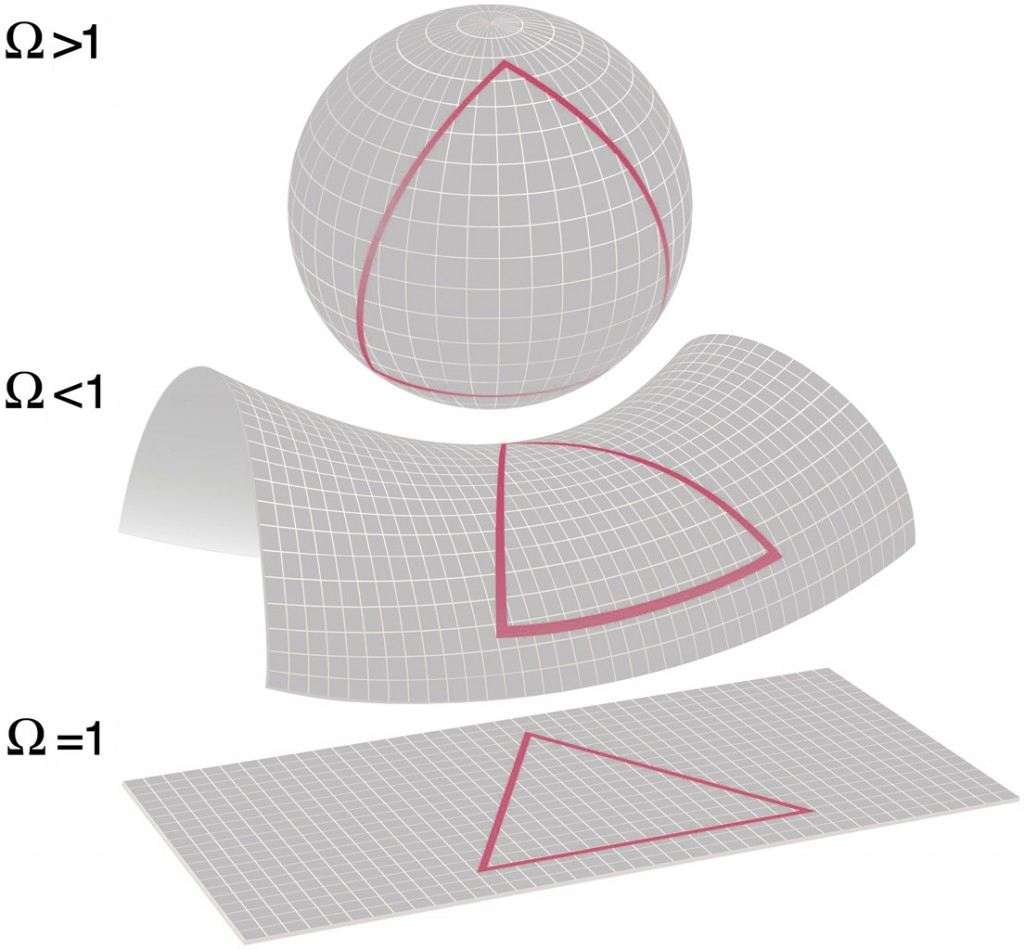
where \(d\Sigma(k)\) refers to the spatial 3-dimentional metric depending on the curvature parameter \(k\) which takes the discrete values +1, 0, -1, corresponding to a closed, open or spacially flat geometry, and we used the normalized form of the scale factor \(a(t) = R(t)/R_0\).
Source: quantum-bits.org
The evolution of the scale parameter as in the case of wavelength (see Exercises):
\[a(t) = \frac{1}{1+z}.\]
Friedman Equations
The dynamics’s of the FLRW metric is governed by the Einstein’s equations. Einstein’s original field equations are:
In Newtonian gravity, the source is mass. In special relativity, is a more general concept called the energy-momemtum tensor, which may be modeled as a perfect fluid for which:
where \(U_\mu\) is the fluid four-velocity in co-moving coordinates, \(\rho\) is an energy density and \(p\) is the isotropic pressure. The FLRW metric solution to the Einstein equations can be reduced to the two Friedmann equations:
where \(i\) stands for the different components of the energy density as we will see later: matter (or dust), radiation, cosmological density, curvature density.
For the special case of \(a(t_0) = 1\), ie, today, we have the formula:
\[H_0^2\Omega_0 = \frac{8\pi G}{3}\rho_0\]
The Cosmological Constant
Einstein was interested in finding \(\dot{a} = 0\) (ie static) solutions. This can be achieved if \(k= + 1\) and \(\rho\) is appropriately tuned. But \(\ddot a\) will not vanish in this case. Einstein therefore modified his equations to:
where the \(\lambda\) term is put in the rhs of the equation as it is interpreted as an effective energy-momentum tensor for the vacuum. With this modification the Friedmann equations become:
The discovery by Hubble that the Universe is expanding eliminated the empirical need for a static world. However, we believe that \(\Lambda\) is actually nonzero, so Einstein was right after all. Assuming that cosmological constant is due to the vacuum energy, most quantum field theories predict a \(\Lambda\) that is 120 orders of magnitude larger than the observational values! this is so-called cosmological constant problem.
Evolution of the Cosmological Constants
In general the energy density will have contributions of distinct components which will evolve differently with the Universe expansion:
Massive particles with negligible velocities are known in cosmology as dust or simply matter. Their density scales as the number density times their rest mass. Their number density scales as the inverse of the volume while the rest mass is constant: \(\rho_M \propto a^{-3}\)
Relativistic particles are known as radiation (although it is not only photons) and their energy density is the number density times the particle energy, the latter is proportional to \(a^{-1}\) (as they redshift with expansion) and so: \(\rho_r \propto a^{-4}\)
Vacuum energy does not change as universe expand so we can define a \(\rho_\Lambda \equiv \frac{\Lambda}{8\pi G} \propto a^0\)
It is useful to pretend that \(-ka^{-2}R_0^{-2}\) represents an effective curvature energy density defining \(\rho_k \equiv -(3k/8\pi G R^2_0)a^{-2}\).
There are good reasons to believe that the energy density of radiation is much less than matter, as photon contrinute only to \(\Omega_r \sim 5 \times 10^{-5}\) mostly in the CMB. Therefore is useful to parametrize the universe today as \(\Omega_k = 1 - \Omega_M - \Omega_\Lambda\).
Direct measures of the Hubble constant.. The most reliable result on the Hubble constant comes from the Hubble Space Telecope Key Project. They use the Cepheids to obtain distances to 31 galaxies (They also use Type Ia Supernovae). A recent study with over 600 Cepheids yielded the number \(H_0 = 73.8 \pm 2.4 \mathrm{\;km\;s^{-1}\; Mpc^{-1}}\). The indirect measurement from Planck Collaboration gives somehow a lower value (this discrepancy as well as the comic distance-ladder method are under investigation).
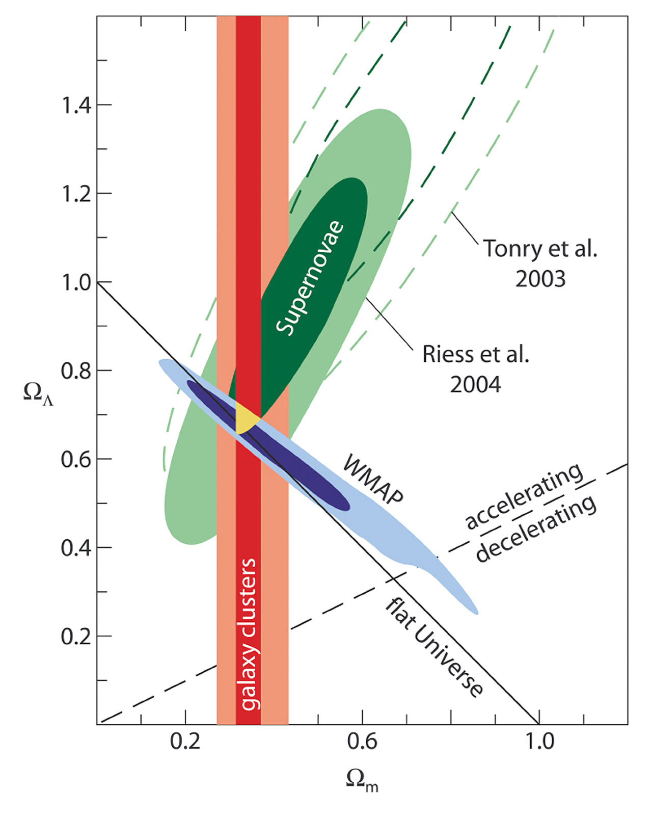
Supernovae. Two major studies, the Supernova Cosmology Project and the High-\(z\) Supernova Search Team, found evidence for an accelerating Universe. When combined with the CMB data indicating flatness (ie \(\Omega_k = 0 \rightarrow \Omega_M + \Omega_\Lambda = 1\)), the best-fit values were \(\Omega_M \approx 0.3\) and \(\Omega_\Lambda \approx 0.7\))
Cosmic Microwave Background. See next section.
Cosmic Microwave Background
The cosmic microwave background (CMB) is electromagnetic radiation that remains from the time when photons decoupled from matter shortly after the recombination of electrons and protons into neutral hydrogen atoms. Once photons decoupled from matter, they traveled freely through the universe without interacting with matter. For an observer today this CMB is observed as a distribution of temperatures (from black body radiation) at on a two-dimensional sphere. This temperature distribution, however, was shown to have anisotropies. If we denote \(\Delta T (\theta, \phi)\) the temperature difference measured in the direction (\(\sin\theta \cos \theta, \sin\theta \sin\theta , \cos\theta\)) with respect to \(T_0 =\) 2.725 K, the average temperature we can decompose these anisotropies over the bases of spherical harmonics, the so called \(Y_{\ell m} (\theta, \phi)\), the same way a we can decompose a function in a curved space over sines and cosines by the Fourier transform:
This decomposition tell us the amount of anisotropy at a given the multipole moment \(\ell\) or angular scale \(\theta = \frac{180^{\circ}}{\ell}\)
\[C_\ell = \langle |a_{\ell m}|^2 \rangle\]
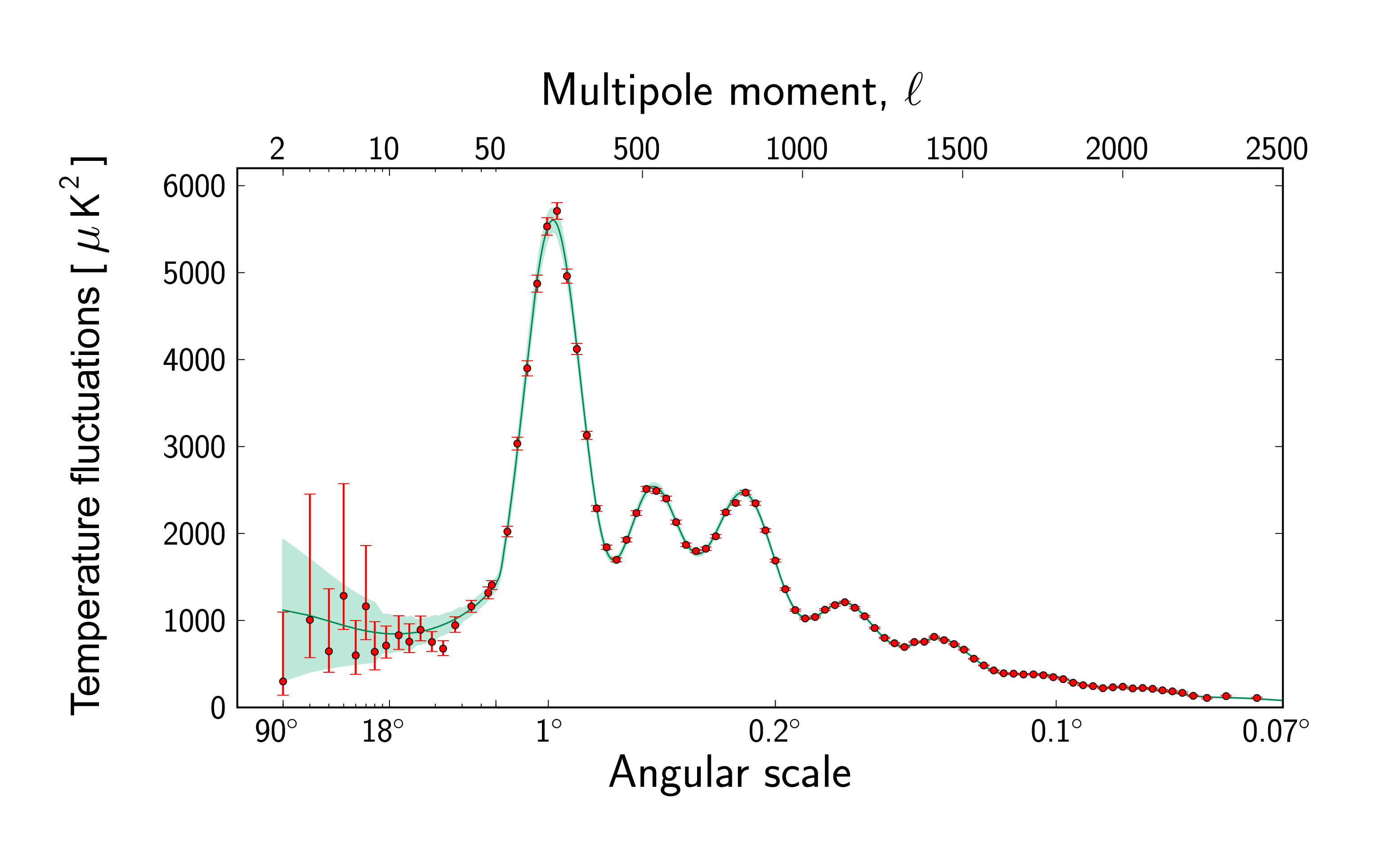
Source: ESA
The power spectrum of the CMB represents the anisotropies of the CMB as a function of the angular scale. The typical spectrum features a plateu at large angular scales (small \(\ell\)) followed by some oscillatory features (aka acoustic peaks or Doppler peak). These peaks represent the oscillation of photon-baryon fuild around the decoupling. The first peak at \(\ell \sim 200\) probes the spatial geometry, while the relative heights probe the baryon density. The position of the first peak constrains the spatial geometry in a way consistent with a flat Universe (\(\Omega_k \sim 0\))
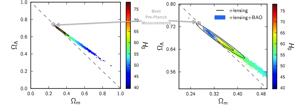
Planck showed that the amount of dark energy in the Universe is appreciably less than we had previously thought, while the amount of dark-and-normal matter is appreciably greater than we thought.
Cosmography
Using the Huble equation we are going to derive some quantities related to the measurement of the Universe.
Age of the Universe
We have shown the evolution of the Hubble expansion as a function of the redshift using the clousure parameters. We know that
Assuming a flat Universe \(\Omega_k =0\) and ignoring the radiation \(\Omega_r \ll \Omega_M\) the integral gets simplified to:
\[H_0 t_0 = \frac{1}{3\sqrt{1 - \Omega_M}}\mathrm{ In}\left(\frac{1+\sqrt{1 - \Omega_M}}{1 - \sqrt{1- \Omega_M}}\right)\] where we used \(1 = \Omega_\Lambda + \Omega_M.\)
For \(\Omega_M = 0.70\) and \(\Omega_\Lambda = (1 - \Omega_M) = 0.30\) one finds \(H_0 t_0 = 0.964\) so that \(t_0 \approx \frac{0.96}{H_0} = 13.5\) Gyr. Which is similar to the assumption we did with a constant \(H_0\).
Comoving distance (Line of Sight)
The comoving distance between two nearby objects in the Universe is the distance between them which remains constant with epoch if the two objects are moving with the Hubble flow. That an object follows the Hubble flow if there is no peculiar velocities, ie, the only reason the 2 objects separate is due to the expansion of the Universe and not because the have relative velocities among them. The comoving distance has the expansion factored out and therefore remains constant with epoch. You can think of it as the distance measured with a ruler that also expands with the Universe. Using the same argument as above with the age of the Universe we can multiplying by the speed of light we can derive:
This is the comoving distance along the line of sight. Ie, is the comoving distance from a galaxy at redshift \(z\) from us. If we want to estimate, let’s say, the distance between 2 galaxies at the same redshift but separated in angle \(\Delta \theta\), then the distance is given by \(D_M \Delta \theta\) where \(D_M\) is the transverse comoving distance. For a flat Universe \(D_M = D_c\) but if the curvature is not zero, the relationship depends on the trigonometric functions \(\sinh\) (for a closed Universe) and \(\sin\) (for an open Universe) to account for the curvature of spacetime.
Luminosity Distances
The luminosity distance defined in cosmology is defined as the distace in which an object with intrinsic luminosity \(L\) is observed with flux \(f\), ie:
\[ f = \frac{L}{4\pi d_L^2}.\]
This in terms of bolometric values, however sometimes we only observe a given bandwidth in frequency, ie, we have to replace \(f\rightarrow f(\nu_o)\) and \(L \rightarrow L(\nu_{e})\) where \(\nu_o\) and \(\nu_e\) are the observed and emitted frequencies. Since the luminosity is defined as energy delivered over interval of time, we can approximate it as:
being \(N\) the number of photos. However the photons emitted are redshifted and photons observed at \(\nu_o\) were emitted at \((1+z)\nu_o\). The time intervals are also related by the expansion of the Universe as:
So we have that the emitted luminosity and the observed luminosity are related as:
\[L(\nu_o) = \frac{L(\nu_e)}{(1+z)^2}.\]
The observed luminosity is smaller than the emitted luminosity. On the other hand the relation between the observed flux and observed luminosity is the same as in a non-expanding Universe. ie:
\[f(\nu_o) = \frac{L(\nu_o)}{4\pi D_c^2},\]
where \(D_c\) is the co-moving distance. Putting everything together we have that:
\[f(\nu_o) = \frac{1}{(1+z)^2}\frac{L(\nu_e)}{4\pi D_c^2} = \frac{L(\nu_e)}{4\pi D_L^2},\] so we have the relation between the luminosity distance and the co-moving distance as:
\[D_L = D_c(1+z).\]
Tutorial IV: Age of the Universe
In the about the age of the Universe we calculated an analytical solution for a given condition. No we are goign to use python to numerically solve the look-back time for any given set of cosmological parameters. For that we are going to rewrite the loopback formula in terms of the scale factor \(a\) since we have the redshift scale relation:
We need to numerically integrate the right hand side of the equation. However, for some parameters this integration is circular, reaching a \(a_{max}\) then the \(H^2(a_{max}) = 0\)
%matplotlib inlineimport matplotlib.pylab as pltplt.rcParams['font.family'] ="STIXGeneral"import numpy as np#Lets use the inline figure format as svg%config InlineBackend.figure_format ='svg'#We take the current value of H0 from the astropy packagefrom astropy.cosmology import Planck13H0 = Planck13.H(0).value#We define the friedman equation ignoring the radiation component omega_r <<def friedman(a, omega_M, omega_lambda): omega_k =1- omega_M - omega_lambda H2 = H0**2* (omega_M * a**-3+ omega_k * a**-2+ omega_lambda)return H2import scipy.integrate as integrate#This is a simple integration, it does not take into account a possible Big Crunch"""def calculate_times(omega_m, omega_lambda): t0 = integrate.quad(lambda x: 1/x * 1/np.sqrt(friedman(x,omega_m, omega_lambda)), 0, 1)[0] times = [] scales = np.arange(0.1, 2, 0.01) for a in scales: time = integrate.quad(lambda x: 1/x * 1/np.sqrt(friedman(x,omega_m, omega_lambda)), 0, a)[0] times.append(H0*(time - t0)) return np.array(times), np.array(scales)"""#This integration takes into account a Big Crunchdef calculate_times(omega_m, omega_lambda):#Lets check if there is a maximal, ie, if H^2(a) = 0 astep =0.001 amax =3 scales = np.arange(0.1, amax, astep) f = friedman(scales, omega_m, omega_lambda) ia, = np.where(np.diff(np.sign(f)))iflen(ia) !=0: amax = scales[ia[0]] tmax = integrate.quad(lambda x: 1/x *1/np.sqrt(friedman(x,omega_m, omega_lambda)), 0, amax - astep)[0]#time today a = 1 t0 = integrate.quad(lambda x: 1/x *1/np.sqrt(friedman(x,omega_m, omega_lambda)), 0, 1)[0]#Empty x,y for the plots times = [] scale = []for a in scales:if a < amax: #If a < amax we do the typical integral 0 -> a time = integrate.quad(lambda x: 1/x *1/np.sqrt(friedman(x,omega_m, omega_lambda)), 0, a)[0] times.append(H0*(time - t0)) #We calibrate at -t0 to place all curves together scale.append(a)if a >= amax and2*amax - a >0: #If a > amax we are out the domain we integrate backwards time =2*tmax - integrate.quad(lambda x: 1/x *1/np.sqrt(friedman(x,omega_m, omega_lambda)), 0, 2*amax - a)[0] times.append(H0*(time - t0)) scale.append(2*amax - a)return np.array(times), np.array(scale)fig, ax = plt.subplots(1, 1, figsize=(5,4))omega_M =0.3omega_lambda =0.7x, y = calculate_times(omega_M, omega_lambda)ax.plot(x, y, label=fr"$\Omega_M =$ {omega_M:.2f}, $\Omega_\Lambda =$ {omega_lambda:.2f}")omega_M =1.0omega_lambda =0x, y = calculate_times(omega_M, omega_lambda)ax.plot(x, y, lw =2, label=fr"$\Omega_M =$ {omega_M:.2f}, $\Omega_\Lambda =$ {omega_lambda:.2f}")omega_M =0.3omega_lambda =0x, y = calculate_times(omega_M, omega_lambda)ax.plot(x, y, lw =2, label=fr"$\Omega_M =$ {omega_M:.2f}, $\Omega_\Lambda =$ {omega_lambda:.2f}")omega_M =4omega_lambda =0x, y = calculate_times(omega_M, omega_lambda)ax.plot(x, y, lw =2, label=fr"$\Omega_M =$ {omega_M:.2f}, $\Omega_\Lambda =$ {omega_lambda:.2f}")plt.legend(loc="upper left")ax.grid()ax.set_xlim(-1,1.5)ax.set_ylim(0.2,2)ax.set_ylabel("$a(t)$")ax.set_xlabel("$H_0 (t - t_0)$")plt.show()
Figure 4.1: Age of the Universe
References
Yañez, Juan Pablo, and Anatoli Fedynitch. 2023. “daemonflux: DAta-drivEn MuOn-calibrated Neutrino
Flux,” February. https://arxiv.org/abs/2303.00022.