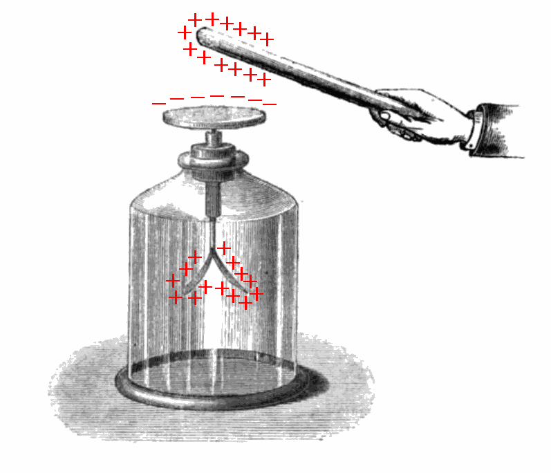
To explain cosmic rays, we need to go back about 100 years to the year 1912 when Victor Hess concluded a series of balloon flights equipped with an electroscope. He measured how ionization in the atmosphere increased as he moved away from the Earth’s surface. The origin of this ionization had to be some type of radiation, and since it increased with altitude, the origin couldn’t be terrestrial. In other words, there existed, and still exdists, radiation coming from outer space. For this milestone, Victor Hess is known as the discoverer of cosmic rays. However, it would be unfair to attribute the merit solely to Hess, as many physicists before him had already paved the way that would culminate in his famous balloon flights: Theodor Wulf, Karl Bergwitz, and Domenico Pacini, among others, laid the foundations for one of the branches of particle physics that would dominate the field for the next 40 years until the advent of the first particle accelerators in the early 1950s.
Electroscope charged by induction. Source: Sylvanus P. Thompson (1881) Elementary Lessons in Electricity and Magnetism, MacMillan, New York, p.16, fig. 12
From the begining, cosmic rays were mysterious: What was their origin? What were these ionizing rays? During the 1920s, Bruno Rossi and Robert Millikan engaged in a lively debate on the nature of cosmic rays. Millikan proposed that cosmic rays were “ultra”-gamma rays, photons of very high energy created in the fusion of hydrogen in space. Rossi’s measurements, showing an East-West asymmetry in the intensity of cosmic rays, suggested instead that cosmic rays must be charged particles, disproving Millikan’s theories. There is a famous anecdote in which Rossi, during the introductory talk at a conference in Rome, said: > Clearly, Millikan is resentful because a young man like me has shattered his beloved theory, so much so that from that moment on, he refuses to acknowledge my existence” A hundred years later, we know that Rossi was indeed correct. The majority, 90%, of cosmic rays are protons and other heavy nuclei. The ratio of nuclei faithfully follows the atomic abundance found in our Solar System, indicating that the origin of these particles is stellar. There are some exceptions; for example, lithium, beryllium, and boron are nuclei that we can find among cosmic rays in a proportion greater than in our environment. These nuclei are actually produced by the fragmentation of heavier ones, such as carbon, during their journey through space. Thus, the abundance ratio between carbon and boron provides information about how long carbon has been traveling through space.
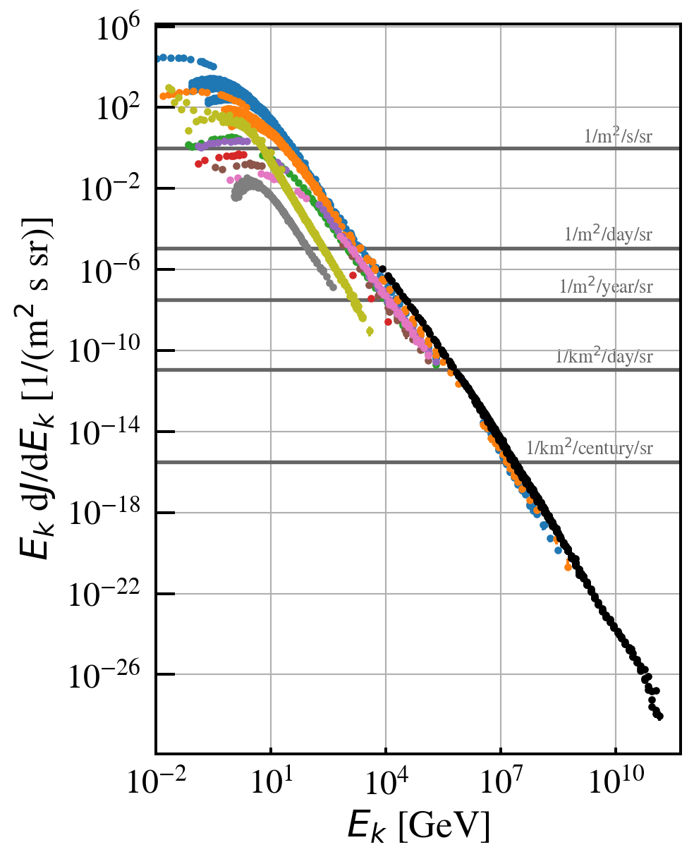
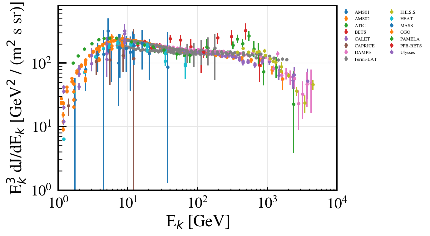
The spectrum, or the number of particles per unit area and time as a function of energy, has also been measured in great detail over the last 30 years thanks to the work of numerous experiments. The cosmic ray spectrum is remarkable in both its variation and energy range. The number of particles, or flux, covers 32 orders of magnitude, so we find that the least energetic particles reach Earth at a rate of one particle per square meter every second. On the other hand, the most energetic ones arrive at a rate of one particle per square kilometer per year. This is why physicists have had to develop various experimental techniques to measure the spectrum of cosmic rays in its entirety: from particle detectors sent into space on satellites or attached to the International Space Station, to experiments deployed on large surfaces of the Earth to detect the most energetic cosmic rays, such as the Pierre Auger Observatory covering an area of about 3000 km2 on the high plateau of the Pampa Amarilla in Malargüe, Argentina.
But what makes cosmic rays truly fascinating is the amount of energy these particles can reach, far superior to what can be achieved today with the most powerful accelerator built by humans with the Large Hadron Collider (LHC) at the European Organization for Nuclear Research (CERN) in Geneva. The LHC is an underground ring with a length of 27 km located on the Franco-Swiss border near Geneva, Switzerland, using powerful magnets to accelerate protons to 99.99% of the speed of light. Despite the impressiveness of this experiment, if we were to accelerate particles to the energies of cosmic rays with the same technology, we would need an accelerator the size of the orbit of Mercury. The speed of cosmic rays is so high that the effects of space-time relativity are considerable. For example, although the radius of our Galaxy is about 100,000 light-years, due to the temporal contraction of special relativity, the most energetic cosmic rays would experience they will experience the journey in just 10 seconds. When cosmic rays reach Earth, they encounter 10 kilometers of atmosphere which, along with the Earth’s magnetic field, fortunately acts as a shield and protects us from radiation. However, when cosmic rays collide with atoms in the atmosphere, they trigger a shower of new particles. This shower is known as secondary cosmic rays, and in it, we can find a diverse array of new particles. This is why, for many years, the physics of cosmic rays was the only way for particle physicists to discover and study new particles. Thus, following in Hess’s footsteps, during the 1940s, many physicists moved from the laboratory to hot air balloons equipped with bubble chambers (a primitive version of a particle detector) to study this myriad of new particles. Among the new particles discovered were, for example, the first particle of antimatter: the positron, a positively charged electron, as well as the muon, with properties similar to the electron but with greater mass.
But what is the origin of cosmic rays? Which sources in the Universe are capable of accelerating particles to such energies? That is the question that, despite 100 years since Victor Hess’s discovery, physicists have not been able to fully answer. The main reason is, however, easy to understand. Cosmic rays, being charged particles, are deflected by magnetic fields during their journey through the Universe. Both the Milky Way and intergalactic space are immersed in magnetic fields, so when cosmic rays reach Earth, their direction has little or nothing to do with the original direction, making it impossible to do astronomy. However, despite this disadvantage, we can deduce some things about their origin based on, for example, their energy. We know that low-energy cosmic rays must come from our own Galaxy because the magnetic fields of the Milky Way would confine them until they eventually interact with Earth. On the other end of the spectrum, extremely high-energy cosmic rays (UHECRs) must come from outside our own Galaxy since they are so energetic that the magnetic fields of their respective galaxies would not be able to retain them. The exact turning point in energy between these two origins is uncertain. So far, we have been unable to undoubtivously observe a cosmic-ray source. One of the main candidates for the source of galactic cosmic rays are supernova remnants. At the end of a star’s life cycle, it can explode, releasing a large amount of mass and energy. What remains behind can be a neutron star surrounded by all the remnants left from the original star; this is what is called a supernova remnant. It is more challenging to conceive a cosmic accelerator capable of accelerating particles up to the energy equivalent of a soccer ball kicked at 50 km/h, which corresponds to the energies of UHECRs. Here the list of candidates is considerably reduced because there are fewer objects in the Universe with the magnetic field and size sufficient to act as a large particle accelerator. The candidates are active galactic nuclei and gamma-ray bursts. Active galactic nuclei are the nuclei of galaxies with a supermassive black hole at their center. These nuclei show beams of particles in opposite directions that could function as large accelerators. On the other hand, gamma-ray bursts are the most violent events known in the Universe, and their origin and nature would warrant another chapter of this book. Lasting from a few seconds to a few minutes, these events can illuminate the entire sky by releasing their energy mainly in the form of very high-energy photons. But if cosmic rays never point to their source, how can we ever be sure that active galactic nuclei or gamma-ray bursts are the true sources of cosmic rays? To answer this puzzle, we need what has been dubbed as multi-messenger astronomy. Thanks to particle physics, we know that under the conditions in which, for example, a proton is accelerated to high energies, reactions with the surrounding matter can occur. These interactions would produce other particles such as very high-energy photons and neutrinos. Neutrinos are especially interesting because they are not only neutral and therefore travel in a straight line without being deflected by magnetic fields, but they are also weakly interacting particles, so unlike photons, they can traverse dense regions of the Universe without being absorbed. Future multi messenger experiments will be able to solve the mystery of cosmic rays.
The Cosmic Ray Spectrum
Cosmic rays mostly protons accelerated at sites within the Galaxy.
As they are charged they are deviated in galactic and inter-galactic \(\vec{B}\) and solar and terrestrial magnetic fields. Directionality only possible for \(E \ge 10^{19}\) eV.
But interactions with CMB at \(E \sim 10^{19}\) limit horizon tens or hundreds of Mpc.
One century after discovery, origins of cosmic rays, in particular UHECR, remain unknown
Code
import crdbimport matplotlib.pylab as pltplt.rcParams['font.family'] ="STIXGeneral"plt.rcParams.update({'axes.labelsize': 20})plt.rcParams.update({'legend.fontsize': 20})plt.rcParams.update({'figure.figsize': [8, 6]})plt.rcParams['xtick.labelsize'] =18plt.rcParams['ytick.labelsize'] =18plt.rcParams['xtick.major.width'] =1.5plt.rcParams['xtick.minor.width'] =1plt.rcParams['xtick.major.pad'] =8plt.rcParams['xtick.direction'] ='in'plt.rcParams['ytick.major.size'] =10plt.rcParams['ytick.minor.size'] =5plt.rcParams['ytick.major.width'] =1.5plt.rcParams['ytick.minor.width'] =1plt.rcParams['ytick.major.pad'] =8plt.rcParams['ytick.direction'] ='in'plt.rcParams['legend.frameon'] =Falseplt.rcParams['lines.linewidth'] =1.5plt.rcParams['axes.linewidth'] =1.5import numpy as npfrom crdb.experimental import convert_energyfig, ax = plt.subplots(1,1, figsize=(5, 7))elements = ("H", "He", "C", "N", "O", "Si", "Fe")elements += ("1H-bar", "e-+e+", "AllParticles")tabs = []for energy_type in ("EKN", "ETOT"):for elem in elements: tab = crdb.query( elem, energy_type=energy_type, energy_convert_level=1, )if energy_type =="EKN": tab = convert_energy(tab, "EK") tabs.append(tab)tab = np.concatenate(tabs).view(np.recarray)#Lets ignore data without systematic errorsmask = (tab.err_sys[:, 0] >0) & (tab.err_sta[:, 0] / tab.value <0.5)tab = tab[mask]ax.set_xlim(1e-2, 5e11)for elem in elements: ma = tab.quantity == elem t = tab[ma]iflen(t) ==0:continue sta = np.transpose(t.err_sta) color ="k"if elem =="AllParticles"elseNone ax.errorbar(t.e, t.value, sta, fmt=".", color=color)ax.loglog()ax.set_ylabel(r"$E_k$ d$J$/d$E_k$ [1/(m$^2$ s sr)]")ax.set_xlabel(r"$E_k$ [GeV]")ax.grid()m =1km =1e3* ms =1sr =1hour =60**2* sday =24* hourmonth =30* dayyear =356* daycentury =100* yearfor flux_ref in ("1/m^2/s/sr","1/m^2/day/sr","1/m^2/year/sr","1/km^2/day/sr","1/km^2/century/sr", ): v =eval(flux_ref.replace("^2", "**2")) label = flux_ref.replace("^2", "$^2$") ax.axhline(y=v, color="0.4", lw =2) ax.text(10**11, v *1.1, label, va="bottom", ha="right", color="0.4", zorder=0, )
Figure 5.1: All particle cosmic ray spectrum
Cosmic Ray as function of…
There are four different ways to describe the spectra of the cosmic ray radiation:
By particles per unit rigidity. Propagation and deflection on magnetic fields depends on the rigidity.
By particles per energy-per-nucleon. Fragmentation of nuclei propagating through the interstellar gas depends on energy per nucleon, since that quantity is approximately conserved when a nucleus breaks up on interaction with the gas.
By nucleons per energy-per-nucleon. Production of secondary cosmic rays in the atmosphere depends on the intensity of nucleons per energy-per-nucleon, approximately independently of whether the incident nucleons are free protons or bound in nuclei.
By particles per energy-per-nucleus. Air shower experiments that use the atmosphere as a calorimeter generally measure a quantity that is related to total energy per particle.
For \(E > 100\) TeV the difference between the kinetic energy and the total energy is negligible and fluxes are obten presented as particle per energy-per-nucleus.
For \(E < 100\) TeV the difference is important and it is common to present nucleons per kinetic energy-per-nucleon. This is the usual way of presenting the spectrum for nuclei with different masses: the conversion in energy per nucleus is not trivial.
Primary Cosmic Rays
The energy spectrum of primary nucleons from GeV to ~ 100 TeV is given by:
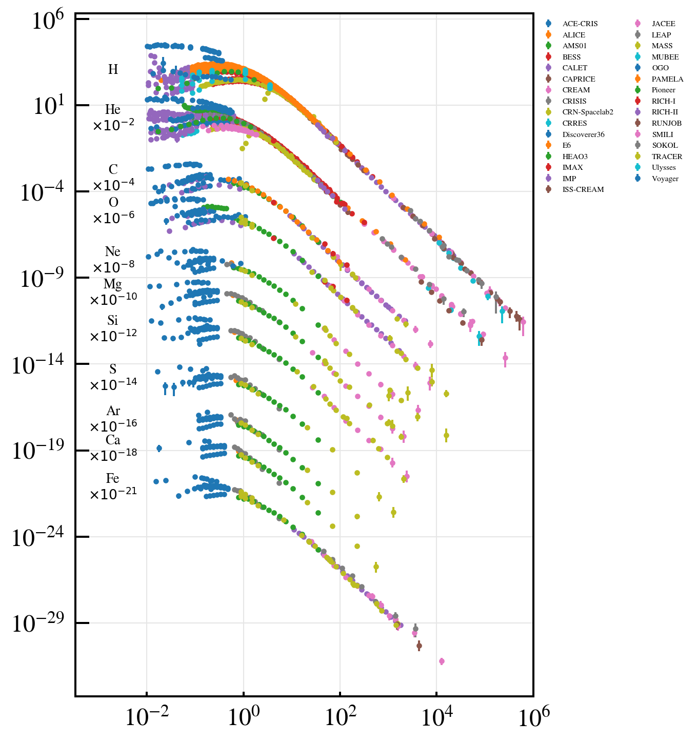
Where \(\alpha \equiv 1+ \gamma = 2.7\) is the differential spectral index and \(\gamma\) the integral spectral index. The composition of the bulk of cosmic rays are: 80% protons, 15% He, and the rest are heavier nuclei: C, O, Fe and other ionized nuclei and electrons (2%)
Code
elements = {"H": 0,"He": -2,"C": -4,"O": -6,"Ne": -8,"Mg": -10,"Si": -12,"S": -14,"Ar": -16,"Ca": -18,"Fe": -21,}xlim =1e-2, 1e6tabs = []for elem in elements: tabs.append(crdb.query(elem, energy_type="EKN"))tab = np.concatenate(tabs).view(np.recarray)# use our energy rangetab = tab[(xlim[0] < tab.e) & (tab.e < xlim[1])]# we don't want upper limitstab = tab[~tab.is_upper_limit]# statistical errors less than 100 %tab = tab[np.mean(tab.err_sta, axis=1) / tab.value <1]# skip balloon datamask = crdb.experiment_masks(tab)["Balloon"]tab = tab[~mask]fig, ax = plt.subplots(1,1,figsize=(6, 9))masks = crdb.experiment_masks(tab)for exp insorted(masks): t = tab[masks[exp]] first =True color =None marker =Nonefor elem, fexp in elements.items(): f =10**fexp t2 = t[t.quantity == elem]iflen(t2) ==0:continue sta = np.transpose(t2.err_sta) l = ax.errorbar(t2.e, t2.value*f, sta*f, fmt=".", color=color, label = exp if first elseNone) first =False color = l.get_children()[0].get_color()for elem, fexp in elements.items(): t = tab[tab.quantity == elem] ymean = np.exp(np.mean(np.log(t[t.e < xlim[0] *100].value))) *10**fexp s =f"{elem}\n$\\times 10^{{{fexp}}}$"if fexp !=0elsef"{elem}" ax.text(2e-3, ymean, s, va="center", ha="center")ax.grid(color="0.9")ax.set_xlim(xlim[0]/30, xlim[1])ax.loglog()ax.legend( fontsize="xx-small", frameon=False, loc="upper left", ncol=2, bbox_to_anchor=(1, 1))#ax.legend()
Figure 5.2: Cosmic Ray spectrum per element
Galactic Cosmic Ray Composition
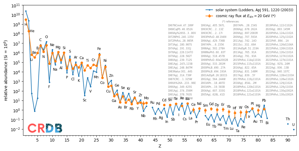
The chemical composition of cosmic rays is similar to the abundances of the elements in the Sun indicating an stellar origin of cosmic rays.
However there are some differences: Li, Be, B are secondary nuclei produced in the spallation of heavier elements (C and O). Also Mn, V, and Sc come from the fragmentation of Fe. These are usually referred as secondary cosmic rays.
The see-saw effect is due to the fact that nuclei with odd Z and/or A have weaker bounds and are less frequent products of thermonuclear reactions.
By measuring the primary-to-secondary ratio we can infer the propagation and diffusion processes of CR.
Cosmic ray composition. Source: CRDB
Electrons
The spectrum of electrons is expected to steepen because the radiative energy loss in the Galaxy. Electrons will lose energy primarly due to synchrotron radiation and inverse Compton scattering
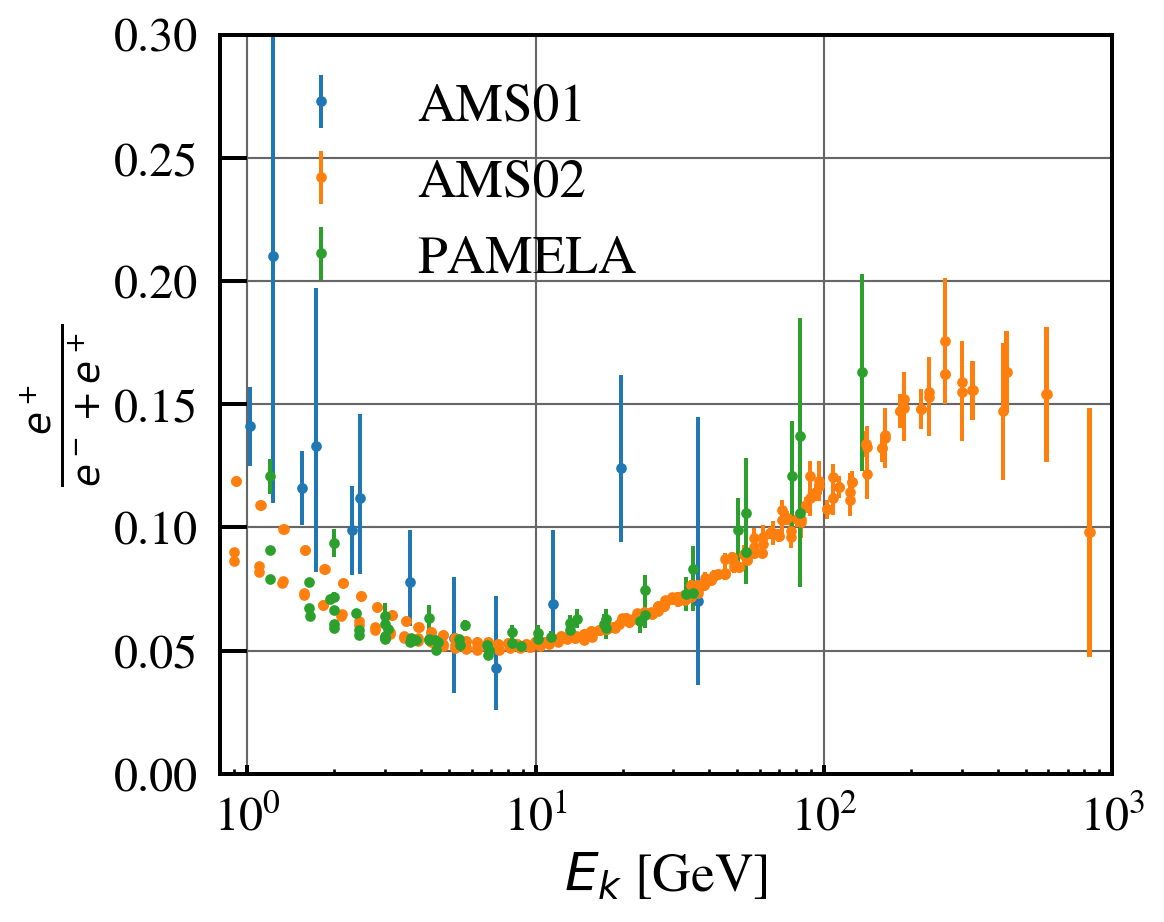
The plot above shows the (\(e^− + e^+\)) spectrum, only PAMELA data refers only to \(e^−\). As can be seen there are several features worth noting:
For \(E \leq\) 20 GeV the spectra is dominated by solar modulations and somehow follows the same spectral index as the proton spectrum, although with factor 0.01 in the normalization, which means that electrons contribute only 1% to the overall CR spectrum.
At about 5 GeV there is a change in the spectrum. Sometimes identified as the energy when electrons start too loose energy, and therefore the spectrum becomes steeper.
For \(E >\) 50 GeV spectra is well fitted with a power law of \(\sim 3.1\) for \(e^−\) and \(\sim 2.7\) for \(e^+\). Since \(e^−\) domimate over \(e^+\) the overall spectrum (\(e^− + e^+\)) also follows a spectral index of \(\sim 3\). Electron spectrum is much steeper than the proton one.
The sum spectrum (\(e^− + e^+\)) has a sharp break at \(E \simeq\) 1 TeV, however this is dominated by the \(e^−\) with an estimate of a ratio of 3 − 4 in \(e^−/e^+\). This cutoff has been confirmed by DAMPE making it the first direct observation of this cutoff.
There is an excess measured by ATIC at \(\sim 700\) GeV. The existance of that feature has, however, never been confirmed by other experiments (Fermi, DAMPE, HESS).
Important
Given the diffusion loss length of electrons is about \(300\;\mathrm{pc}\) and confinement time in the Galaxy about \(100\;\mathrm={yrs}\) it is assumed that the electron spectrum above few TeV is dominated by nearby and young cosmic ray sources.
Question
Assuming the electron flux is only 1% of the protons. Is it the Earth positive charged-up?
Antimatter
As antimatter is rare in the Universe today, all antimatter we observe are by-product of particle interactions such as Cosmic Rays interacting with the interstellar gas.
The PAMELA and AMS-02 satellite experiments measured the positron to electron ratio to increase above 10 GeV instead of the expected decrease at higher energy.
This excess might hint to to contributions from individual nearby sources (supernova remnants or pulsars) emerging above a background suppressed at high energy by synchrotron losses.
6 Galactic Cosmic Rays
Propagation of Cosmic Rays
One trivial argument to discriminate between a Galacic or extra-Galactic origin of the origin of cosmic rays is to check whether or not the larmor radius, \(r_L\), of cosmic ray particles is of the order of the size of the Galaxy. As we showed, we can express the larmor radius as:
There are many uncertainties in these numbers but we can assume that the size of the Galactic halo is \(h \sim 1 - 10\; \mathrm{kpc}\), and the magnetic field in the halo is about \(B \sim 0.1 - 10 \;\mu\mathrm{G}\). Putting this number gives maximum energy of \(E_{max} \sim 10^{17} - 10^{20} \;\mathrm{eV}\). Given this result we can assume that lower energy cosmic rays come from own Galaxy, otherwise they would have escaped.
Cosmic-ray Interactions
Since the bluck of cosmic-ray particles are expected come from the Galaxy we can now evaluate where and how they will interact during their travel. There are two chiefly process in which a cosmic-ray particle can interact:
Coulomb collissions: They occur when a particle interacts with another particle via electric fields.
The Coulomb cross-section for a 1 GeV particle is \(10^{-30} \; \mathrm{cm}^2\).
For 1 GeV cosmic-ray propating in the ISM (\(n \sim 1 \; \mathrm{cm}^{-3}\)) the mean Coulomb interacion length rate is \(1/n\sigma \sim 324100 \; \mathrm{Mpc}\) which is much larger than the Galaxy size. Therefore coulomb collisions can be neglected.
Spallations processes: It occurs when C, N, O, Fe nuclei impact on intestellar hydrogen. The large nuclei is broken up into smaller nuclei. A clear indication of a spallation comes precisely from the composition comparison with stellar matter.
sigma =1e-30#in cm2n =1# in cm-3l =1./(n*sigma) *3.241e-25# in Mpcprint (f"The interaction length for Coulomb collisions is {l:.2} Mpc")
The interaction length for Coulomb collisions is 3.2e+05 Mpc
The Interstellar Medium (ISM)
Given the low density of the Galactic halo it is clear that the spallation processes must occur in the Galactic Disk. The Galactic Disk is mostly populated by the Interstellar Medium or ISM. It is mostly composed by Hydrogen in 3 different phases:
Molecular Gas. This phase is the more clumpsy as they gathered in molecular clouds that can reach densities of \(10^{6} \; \mathrm{cm}^{-3}\) which is still very low for our atmosphere standards (14 lower). It is composed of hydrogene in molecular form, \(\mathrm{H}_2\), \(\mathrm{CO}\). Sometimes called stars nurseries they are stars forming regions.
Atomic Gas. Made up of neutral atomic Hydrogen (HI in astronomical nomenclature). The maps tracing the \(\mathrm{HI}\) that is organized in a spiral pattern, like \(\mathrm{H}_2\), and also its structure is quite complex, with overdensities and holes.
Ionized Gas. Is ionized Hydrogen or \(\mathrm{HII}\).
The overall density of the ISM is \(\sim 0.1-1 \;\mathrm{cm}^{-3}\). The interstellar gas is not a an static gas, but rather is subject to a turbulent motion.
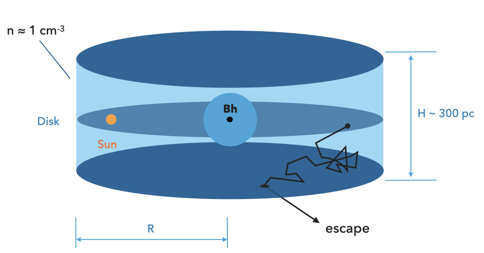
The Leaky Box Model
The Leaky Box model is a very simple model used to describe cosmic-ray confinement. In this simplified phenomenological picture CRs are assumed be accelerated in the galactic plane and to propagate freely within a cylindrical box of size \(H\) and radius \(R\) (see Figure 6.1) and reflected at the boundaries; the loss of particles is parametrized assuming the existence of a non-zero probability of escape for each encounter with the boundary (Poisson process).
Figure 6.1: Representation of the leaky box model of the Galaxy
Primary-to-Secondary Ratios
Since we know the partial cross-section of spallation processes we can use the secondary-to-primary abundance ratios to infer the gas column density traversed by the average cosmic ray.
Let us perform a simply estimate of the Boron-to-Carbon ratio. Boron is chiefly produced by Carbon and Oxygen with approximately conserved kinetic energy per nucleon (see Superposition principle), so we can relate the Boron source production rate, \(Q_B(E)\) to the differential density of Carbon by this equation:
\[Q_B(E) \simeq n_{ISM} \beta c \sigma_{f,B} N_C\]
where, \(n_{ISM}\) denotes the average interstellar gas number density and \(N_C\) is the Carbon density and \(\beta c\) is the Carbon velocity and \(\sigma_{f,B}\) is the spallation or fragementation cross-section of Carbon into Boron.
The Boron disappears by escaping the galaxy in Poisson process or lossing its energy. The disappearence of Boron can be written using a lifetime \(\tau\) as:
\[D_B = \frac{N_B}{\tau}\]
assuming the amount of Boron in the Galaxy is constant per unit time, \(\dot{N}_B = 0\), then the production of Boron has to be equal to the disappearence rate, in other words: \[\dot{N}_B = 0 = Q_B - D_B\]
We can write:
\[\frac{N_B}{N_C} \simeq n_{H} \beta c \sigma_{\rightarrow B}\tau\]
Boron-to-Carbon Ratio
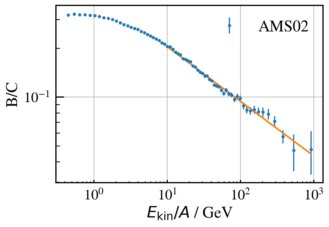
The plot below represents the latest measurements from PAMELA and AMS satellites of the Boron-to-Carbon ratio. The decrease in energy of the Boron-to-Carbon ratio suggests that high energy CR spend less time than the low energy ones in the Galaxy before escaping.
Code
tab = crdb.query("B/C", energy_type="EKN")# select only entries with systematic uncertaintiesmask = tab.err_sys[:, 1] >0tab = tab[mask]fig, ax = plt.subplots(1, 1, figsize=(6,5))from matplotlib import pyplot as plt# Let's plot AMS02 onlyfor i, (exp, mask) inenumerate(crdb.experiment_masks(tab).items()): t = tab[mask] sta = np.transpose(t.err_sta) ax.errorbar(t.e, t.value, sta, fmt=".", label=exp)ax.legend(ncol=2, frameon=False)ax.grid()ax.set_xlabel("$E_\\mathrm{kin} / A$ / GeV")ax.set_ylabel("B/C")ax.loglog()
Figure 6.2: B/C ratio
Tutorial I: Fit the B/C spectrum of AMS-02 data
We are going to retrive the data and fit it. We are going to use python to download the data
tab = crdb.query("B/C", energy_type="EKN")# select only entries with systematic uncertaintiesmask = tab.err_sys[:, 1] >0tab = tab[mask]fig, ax = plt.subplots(1, 1, figsize=(6,4))from matplotlib import pyplot as plt# Let's plot AMS02 onlyfor i, (exp, mask) inenumerate(crdb.experiment_masks(tab).items()):if exp =="AMS02": t = tab[mask] sta = np.transpose(t.err_sta) ax.errorbar(t.e, t.value, sta, fmt=".", label=exp)#Let's use a simple linear model in log-logdef model(x, a, b):return a + b * xfrom scipy.optimize import curve_fit#We only fit in the linear part, ie when E > 10 GeV and we ignore statistical errors. mask = t.e >10popt, pcov = curve_fit(model, np.log10(t.e[mask]), np.log10(t.value[mask]))ax.plot(t.e[mask], np.power(10, model(np.log10(t.e[mask]), popt[0], popt[1])), linewidth=2)ax.legend(ncol=2, frameon=False)ax.grid()ax.set_xlabel("$E_\\mathrm{kin} / A$ / GeV")ax.set_ylabel("B/C")ax.loglog()print(f"The values are \u03B1 = {10**popt[0]:.2} and \u03B2 = {popt[1]:.2}")
The values are α = 0.44 and β = -0.34
Boron to Carbon ratio
Above about 10 GeV/nucleon the experimental data can be fitted to a test function, therefore the Boron-to-Carbon ratio can be expressed as:
\[\frac{N_B}{N_C} = n_{H}\beta c \sigma_{f,B} \tau =0.4 \left(\frac{E}{\mathrm{GeV}}\right)^{-0.3}\]
For energies above 10 GeV/nucleon we can approximate \(\beta \sim 1\), which leads, using the values of the cross-section, to a life time gas density of:
But what is this Boron lifetime? The lifetime \(\tau\) for Boron includes the catastrophic loss time due to the partial fragmentation of Boron, \(\tau_{f,B}\) and the escape probability from the Galactic confinement volume, \(T_{esc}\). The fragmentation cross section is \(\sigma_{f,B} \approx 250\) mbarn so we find that:
which is a good match with the loss time bound at \(\sim\) 1 GeV but is larger at higher energies and does not depend on energy. For example at 1 TeV it is an order of magnitude larger:
which is too small compared to the effective lifetime found. This seems to indicate that CR do not travel in straight lines. Let’s assume that the overall process is a convination of both the borom fragmentation and another process with a lifetime \(T\). By summing the inverse of these processes (being exponential processes):
There no other physical loss process for Boron, so \(T\) really must be the escape of the galactic confinement (leaky box). But if the box has a size \(H\), \(T_{esc}\) will be H/c which is the time required by CR generated in the Galactic plane to escape the box of height \(H\)! However we know that \(T \gg H/c\). So there must be something else confining the CR in the galaxy… what could it be?
Dynamics of Charge Particles in Magnetic Fields.
Before solving the problem what process in the Galaxy is confining the cosmic-rays, let’s review a bit the dynamics of charge particles in magnetic fields.
Let’s assume the simplest case of a test particle or mass \(m_0\) and charge \(Ze\) and lorentz factor \(\gamma\) in an uniform static magnetic field, \({\mathbf B}\).
In a magnetic field the acceleration is always perpendicular to \({\mathbf v}\) so \({\mathbf v\cdot a} = 0\) resulting in:
\[m_0\gamma\frac{d{\mathbf v}}{dt} = Ze ( {\mathbf v} \times {\mathbf B})\]
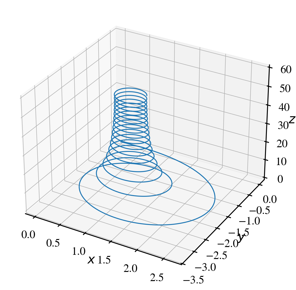
This equation tell us that there is no change in the \(v_{\parallel}\) the parallel component of the velocity and the aceleration is only perpendicular to the magnetic field direction, \(v_{\perp}\). Beacuse \({\mathbf B}\) is constant this results in a spiral motion around the magnetic field. Now we are going to test what happens if the magnetic field is not uniform.
Tutorial II: Motion of a charge particle in a slowly changing magnetic field
The picture above holds while the gyroradius is larger or smaller than the variation of the magnetic field. In the first case when \(R_g \ll (\Delta B)\) the charge particle will follow the substructure of the magnetic field. In the second case \(R_g \gg (\Delta B)\) the magnetic field irregularities are transparent to the particle. However when \(R_g \approx (\Delta B)\) then the particle sees the magnetic irregularities. In this case the particle will scattered almost inelastically in this irregularities. The picture of a test-particle moving in a magnetic field is a simplistic one. In reallity cosmic ray particles propagate in collisionless, high-conductive, magnetized plasma consisting mainly of protons and electrons and very often the energy density of cosmic ray particles is comparable to that of the background medium. As a consequence of that, the electromagnetic field in the system is severely influenced by the cosmic ray particles and the description is more complex than the motion of a test charged particle in a fixed electromagnetic field. This will generate irregularities in the magnetic field. The irregularities in the Galactic magnetic field are responsible for the diffusive propagation of cosmic rays.
Diffusion of Cosmic Rays
The results above leads to think that CR experience diffusion in the galaxy. The equation that we used to relate the Boron production rate by the Carbon spallation process can be seen as a diffuse equation.
In diffusion the continuity equation states that the variation of the density \(N\) in time is given by its transfer of flux in area plus the source contribution:
We made use of the fact that the escape probability is constant per unit time (Poisson process) and so the distribution in time can be writen as:
\[N_i(t) = n_0 e^{-\frac{t}{T_{esc}}}\]
In the absent of collisions and other energy changing processes, the distribution of cosmic ray path lengths can also be written as:
\[N_i(z) = n_0 e^{-\frac{z}{H}}\]
with \(z\) the travel distance in the z-axis and \(H\) the heigth of the box. Using both expressions of the cosmic ray distribution (in time and in space), together with the diffusion formula above give us equation:
\[T_{esp} = \frac{H^2}{D} \]
However we found from the B/C ratio that \(T_{esc} \propto E^{-\delta}\) with \(\delta = 0.55\), therefore the diffusion coefficient is:
\[ D(E) \propto E^{\delta} \sim E^{0.55}\]
Note that physically \(D = D(z)\) ie, diffussion will depend on distance to the disc, however in the leaky-box model we assumed that \(D\) is independent of that, which it is only an approximation.
The State-of-Art of Diffusion
The leaky box model is a very simplistic approximation but more realistic diffusion models, such as the numerical integration of the transport equation in the GALPROP code (Strong and Moskalenko 1998), lead to results for the major stable cosmic-ray nuclei, which are equivalent to the Leaky-Box predictions at high energy. However sofisticated models of transport should include effects such as:
Diffusion coefficient non spatially constant.
Anisotropic diffusion (Parallel vs Perpendicular)
Effect of self-generation waves induced by CR.
Damping of waves and its effects in CR propagation
Cascading of modes in wavenumber space
Each of these effects might change the predicted spectra and CR anisotropies in significant ways.
Transport Equation on Primary Cosmic Rays
The general simplified transport/dissusion equation that relate the abundances of CR elements can be given by:
\[\frac{\partial N_i(E)}{\partial t} =\frac{N_i(E)}{T_{esc}(E)} = Q_i(E) - \left(\beta c n_H \sigma_i + \frac{1}{\gamma\tau_i}\right)N_i(E) + \beta c n_H \sum_{k\ge i}\sigma_{k\rightarrow i}N_K(E)\]
where now \(Q_i(E)\) is the local production rate by a CR accelerator, the middle part reprensents the losses due to interactions with cross-section \(\sigma_i\) and decays for unestable nuclei with lifetime \(\tau_i\). The last term is the feed-down production due to spallation processes of heavier CR. We can simplified this equation depending if we are dealing with Primary or Secondary CR:
Secondaries \(\rightarrow\) neglect production by sources: \(Q_s = 0\)
For example, let’s assume now a primary CR, \(P\), where feed-down spallation is not taking place (ie, they are not product of heavier CR) and no decay (most nuclei are stable, one exception is \(^{10}\)Be which is unstable and \(\beta\)-decay), the equation can be written as:
\[\frac{N_P(E)}{T_{esc}(E)} = Q_P(E) - \frac{\beta c \rho_H N_P(E)}{\lambda_P(E)} \rightarrow N_P(E) = \frac{Q_P(E)}{\frac{1}{T_{esc}(E)}+\frac{\beta c \rho_H}{\lambda_P(E)}}\]
where we wrote \(n_H = \rho_H/m\) and \(\lambda_P\) is the mean free path in \(\mathrm{ g / cm}^2\).
While \(T_{esc}\) is the same for all nuclei with same rigidity, \(\lambda_i\) is different and depends on the mass of the nucleus. The equation suggests that at low energies the spectra for different nuclei will be different (eg for Fe interaction dominates over escape) and will be parallel at high energy if accelerated on the same source. For proton with interaction lengths \(\lambda_{proton} \gg \lambda_{esc}\) at all energies so the transport equation gets simplified to:
\[N_{p}(E) = Q_p(E)\cdot T_{esc}(E)\]
ie, we observe at Earth a proton density of \(N_p(E)\propto E^{-(\gamma +1)} \sim E^{-2.7}\), and \(T_{esc}(E)\) goes with the inverse of the diffusion coefficient \(D(E)\), ie \(T_{esc}(E) \propto E^{-\delta}\), then at the production site the spectrum must follow \(Q_p(E) \propto E^{-\alpha}\) with:
\[\alpha = (\gamma + 1) -\delta \approx 2.1\]
Acceleration of Galatic Cosmic Rays
Three questions:
What is the source of power?
What is the actual mechanism?
Can it reproduce the spectral index found? ### Energy density of galactic cosmic-rays
In cosmic ray physics we called spectrum to the flux per stero radian, so the relationship between them is:
import scipy.constants as ctefrom astropy.constants import pccspeed = cte.value("speed of light in vacuum") *1e2# in cm/semin =1.#GeVemax =1e5# 100 TeVrho =4* np.pi /cspeed *1.8/ (1-1.7) * (np.power(emax,1-1.7) - np.power(emin,1-1.7)) *1e9# in ev cm-3print(r"The energy density is $\rho_{CR} \approx %.2f$ $\mathrm{ ev/cm}^{3}$"%rho)
The energy density is $\rho_{CR} \approx 1.08$ $\mathrm{ ev/cm}^{3}$
This energy density is comparable with the energy density of the CMB \(\rho_{CMB} \approx 0.25\) eV/cm\(^{3}\)
Required Power for Galactic Cosmic Rays
If we assume this value to be the constant value over the galaxy, the power required (called luminosity in astrophysics) to supply all the galactic CR and balance the escape processes is:
R =15000* pc.to("cm").value # radius in Cmh =300* pc.to("cm").valueVd = np.pi * R **2* hprint(r"Galactic Volume is %.1e $\mathrm{ cm}^{-3}$"%Vd)evtoerg = cte.value("electron volt-joule relationship") *1e7tesc =1e14# s cm^3 at 1 GeVtesc = tesc/0.1# spower = (Vd * rho) * evtoerg / tescprint(f"Power L ~ {power:.2e} erg /s")
Galactic Volume is 6.2e+66 $\mathrm{ cm}^{-3}$
Power L ~ 1.08e+40 erg /s
It was emphasized long ago (Ginzburg & Syrovatskii 1964) that supernovae might account for this power. For example a type II supernova gives an average power output of:
Therefore if SN transmit a few percent of the energy into CR it is enough to account for the total energy in the cosmic ray beam. That was called the SNR paradigm
Power Required for > 100 TeV
The derivation above was considered using the CR flux with an integral spectral index of \(\gamma = \alpha -1 = 1.7\) which describes well the CR up to the knee (See Section 6.1). This is the bulk of cosmic ray density. The power required for the high energy part will be significantly less due to the steeply falling primary cosmic ray spectrum. For example assuming an integral index of \(\gamma = 1.6\) for \(E < 1000\) TeV and \(\gamma = 2\) for higher energy we get:
\[\begin{aligned}
\sim 2 \times 10^{39} {\;\mathrm{\;erg/s\; for\;} } E &> 100 \mathrm{\; TeV}\\
\sim 2 \times 10^{38} {\;\mathrm{\;erg/s\; for\;} } E &> 1 \mathrm{\;PeV}\\
\sim 2 \times 10^{37} {\;\mathrm{\;erg/s\; for\;} } E &> 10 \mathrm{\;PeV}
\end{aligned}\] ` which are considerably less than the total power required for all the cosmic-rays. This power might be available from a few very energetic sources.
Fermi Acceleration
Fermi studied how it is posible to transfer macroscopic kinetic energy of moving magnetized plasma to individual particles. He considered an iterative process in which for each encounter a particle gains energy which is proportional to the energy.
Let’s write the increase in energy as \(\Delta E = \xi E\) after \(n\) encounters then:
\[E_n = E_0(1 + \xi)^n\]
where \(E_0\) is the injection energy in the acceleration region. If the probability of escaping this acceleration region is \(P_{esc}\) per encounter, after \(n\) the remaining probability is \((1 - P_{esc})^n\). To reach a given energy \(E\) we need:
after each interaction there is a fraction \((1-P_{esc})\) that remain and the rest escapes the accelerator. If \(N_0\) particles entered the “encounter” in the first place, after \(n\) interaction those remaining are:
\[N(\ge E_n) = N_0(1- P_{esc})^n\]
These particles will always eventually escape since \(P_{esc}\) is not 0, but for any given number of cycles, \(n\), we can be sure that those remaining particles (whenever they escape) will have more energy than those that escaped at the cycle \(n\). We can rewrite:
where \(T_{cycle}\) is the characteristic time of acceleration cycle, and \(T_{esc}\) is the characteristic time to escape the acceleration region.
Note that \(N(\ge E)\) is the integral spectrum, the differntial spectrum is given by:
\[ n(E) \propto E^{-1 - \gamma} \]
Fermi Mechanism
A mechanism working for a time \(t\) will produce a maximum energy:
\[E\leq E_0 (1+\xi)^{t/T_{cycle}}\]
Two characteristic features are apparent from this equation:
High energy particles take longer to accelerate
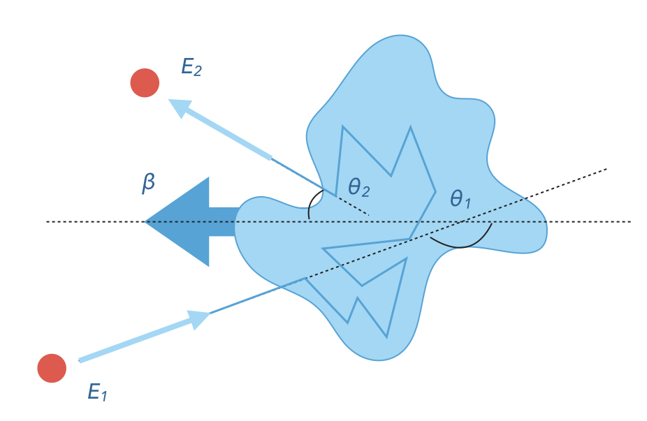
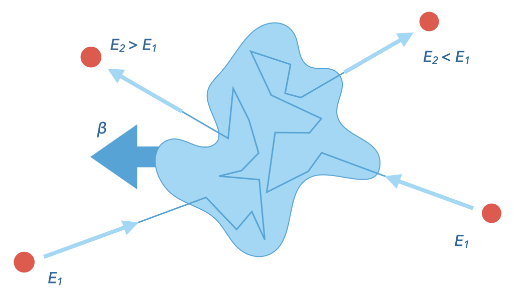
If a given kind of Fermi accelerator has a limited lifetime this will be characterize by a maximum energy per particle that can produce. In the general mechanism we can imagine a particle encountering something moving at a speed \(\beta\). This “something” can be for example a magnetic cloud.
In this general approach, the particle might enter at different angles and exit at difference angles. Let’s assume \(O^\prime\) to be the reference system where the magnetic cloud is in the rest frame. A particle with energy \(E_1\) in the lab reference system will have total energy in this reference system given by the boost transformation with \(\beta\) being the speed of the plasma flow (cloud:
As the particle suffers from colissioness scatterings inside the cloud the energy in the moving frame just before it escapes is \(E_2^\prime = E_1^\prime\) and so we can calculate the increment in energy \(\Delta E = E_2 - E_1\) as:
In the second order (first chronologically) Fermi considered encounters with moving clouds of plasma.
The scattered angle is uniform so the average value is \(\langle \cos\theta_2^\prime\rangle = 0\).
The probability of collision at angle \(\theta\) with the cloud of speed V is proportional to the relative velocity between the cloud and the particle \(c\) if we assume it relativistic (factor \(1/2\) is there to have a proper normalization):
The energy increase is second order of \(\beta\) and..
… the random velocities of clouds are relatively small: \(\beta \sim 10^{-4}\) !!!
Some collisions result in energy losses! Only with the average one finds a net increase.
Very little chance of a particle gaining significant energy!
The theory does not predict the power law exponent
Fermi 1st Order Acceleration.
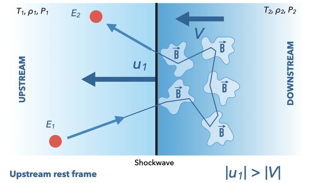
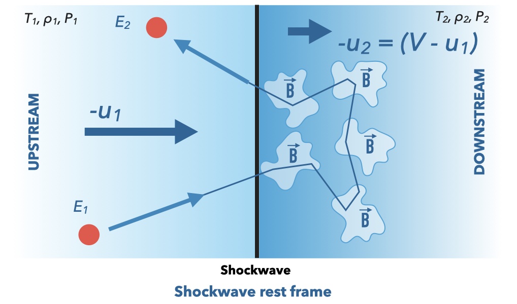
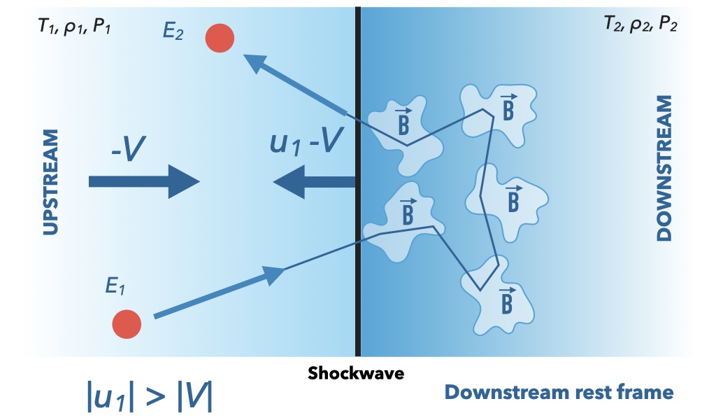
Let’s imagine a shock moving through a plasma. In the reference system of the unshocked plasma the shock front approaches with speed \(\vec{u_1}\) while the shocked plasma (left behind) moves at a slower velocity \(\vec{V}\) where \(|V| < |u_1|\). If we now changed to the reference system where the shock-front is at rest the gas unshocked now appears to approach speed \(-\vec{u_1}\) while the shocked plasma recedes with speed \({-\vec u_2 = (\vec{V} - \vec u_1)}\). A test cosmic ray particle crossing from any side of the shock, will always face an encounter with plasma aproaching at speed \(|V|\), hence \(\beta\) now refers to this speed, the speed of the shocked (downstream) gas in the upstream reference system.
(a) Upstream
(b) Shockwave
(c) Downstream
Figure 6.3: Fermi first order acceleration. Different referenec systems.
The outcoming distribution of particles is not now 0, there is an asymmetry in the Fermi shock acceleration model, as particle in the upstream will re-enter the shock, only those going downstream can escape. Therefore the distribution follows the projection of an uniform flux on a plane:
The incoming angle distribution is also the projection of an uniform flux on a plen but this time with \(-1 \leq \cos\theta_1 \leq 0\) and so \(\langle \cos \theta_1 \rangle = -2/3\)
Particles entering the shockwave and exiting will have a gain of:
The escape probability of loss rate of particles is given by the ratio of the incoming flux and the outgoing flux of particles.
Incoming rate. Let’s assume that the diffusion of particles is so effective that close to the shockwave the distribution of particles is isotropic. In this case the rate of encounters for a plane shock is the projection of an isotropic flux onto the plane shock. Let’s assume \(n\) to be the density of particles close to the shock, because it is isotropic it should follow:
assuming the particles moving at relativistic speed, the velocity across the shock is \(c\cos\theta\) therefore the rate of encounters of particles upstream with the shock is given by:
\[R_{in} = \int \mathrm{ d} n c \cos\theta = \int_0^1 \mathrm{ d} \cos \theta \int_0^{2\pi} \mathrm{ d} \phi\frac{cn(E)}{4\pi}\cos\theta = \frac{cn(E)}{4}\]
where \(n(E)\) is the CR number density.
Outgoing rate. The outgoing rate is simply the number of particles escaping the system. In the shock rest frame, that’s all particles not returning to the shockwave. In this reference system there is an outflow of cosmic-rays adverted downstream. Since particles are diffusing in all direction, the net outflow goes with the velocity of the downstream speed and is given simply by \(R_{out} = n(E) u_2\),
So we get an estimate of the spectral index based on the relative velocities of the downstream and upstram gas in the sockwave.
Kinematic Relations at the Shock
In order to derive the exact value of the spectral index we need to obtain a relation between \(u_1\) and \(u_2\) using the kinematics of a shock wave. This equations are the conservation of mass, the Euler equation for momentum conservation and conservation of energy:
where this equation accounts for the kinetic, internal, and potential energy \(\Phi\).
Let’s assume a one-dimensional, steady shock in its rest frame (otherwise time derivates must be taking into account).
Then the first equation becomes simply: \[\frac{d}{dx} (\rho u) = 0\]
and the Euler equation simplifies to:
\[\frac{d}{dx}(P + \rho u^2) = 0\]
In the energy equation we assume \(\Phi = 0\):
\[\frac{d}{dx}\left(\frac{\rho u^3}{2} + (\rho U + P)u\right) = 0 \]
\[\frac{d}{dx}\left[ \rho u \left(\frac{u^2}{2} + U + \frac{P}{\rho}\right) \right] = 0 \]
where \(U\) is the internal density per unit volume and we can write \(\rho U = \frac{P}{\Gamma -1}\), where \(\Gamma = c_p/c_v\) is the adiabatic index or heat capacity ratio.
Conditions of discontinuity at the shochwave
Let’s assume we are in the shock ref system. Applyting these equations at the discontinuity of the shock we have the three conditions at the discontinuity of the shock:
For a gas with \(P = K \rho^\Gamma\) the speed of sound can be written as \(c_s = \sqrt{\Gamma P / \rho}\) or \(\rho c_s^2 = \Gamma P\). From the second condition we can write:
Which matches remarkably to what we derived to be the differential spectral index at the accelerator:
\[ n(E) \propto E^{-(\gamma+1)} \sim E^{-2.1} \]
Maximum Energy
In an infinite planar shockwave, all particles upstream will encounter again the shochwave. However particles can advent downstream. In diffuse shock accelerations, particules will diffuse travelling a distance \(l_D\) upstream, until they are reached by the shock moving at spead \(u_1\) in the upstream reference system. Particles will cross when:
where we can assume \(t_d\) to be the time during which the mechanism is working, ie the livetime of the shockwave \(t_d \sim t_{age}\). From the equation above we can conclude that the maximum energy:
increases with time
depends on: age, shock speed, magnetic field intensity and structure (through D)
is not universal
\(D\) and therefore \(l_d\) increases with energy, and the each cycle energy increases, so the last cycle is the longest
We can rewrite the diffusion coefficient as: \[ D \sim \frac{l_d^2}{t_d} = l_d v \] where \(v\) is the particle speed. A more detailed analysis gives \(D = \frac{1}{3}l_d v\) where the factor 3 comes from the 3 dimensions. In other words, the diffussion coefficient can be understood as the product of the particle velocity \(v \simeq c\) and its mean free path. At high energies, the mean free path between scatterings in the turbulent magnetic clous can be approximate as \(l_d = r_L/r_0\), where \(r_0\) is the size of the magnetic cloud and \(r_L\) the Larmor radius of the particle. Assuming that \(r_L \gg r_0\) we can re-write:
\[ D = \frac{r_L c}{3} \sim \frac{1}{3}\frac{E c}{Z eB} \]
Another way to see this, is to assume that mean diffusion path \(l_d\) cannot be smaller than the Larmor radius, since a magnetic field irregularities in a smaller scale than the Larmor radisu will be transparent. This is the regime of the Bohm diffusion and it is possible in higly turbulent magnetic fields, something that theoreticians think is possible when CR excite magnetic turbulence at shocks while being accelerated. This is called magnetic field amplification.
In that case, the diffusion coefficient depends linearly with energy (\(\alpha = 1\)) and the equation above can be rewritten as:
\[E_{max} \leq 3 \frac{u_1}{c} Z e B (u_1 t_{age})\]
where \(t_{age}\) is the time in which the accelerator is working. Note that the product \((u_1 t_{age})\) is the radius of a expanding shell. Using some estimates on the time (\(t_{age} \sim\) 1000 yrs as the typical SN shockwave) and \(B_{ISM} \sim 3 \mu\)G we can rewrite the maximum energy for SN shockwaves as:
In order words, the shock-wave acceleration shown can accelerate CR up to 100 Z TeV, but not beyond this. Other acceleration mechanism are needed for the highest energy cosmic rays. We need very high magnetic fields (non-lineal acceleration mechanism). In these cases, even if this object cannot supply the all the galactic cosmic rays the energy per particle may be orders of magnitude higher than those possible in shock acceleration by blast waves.
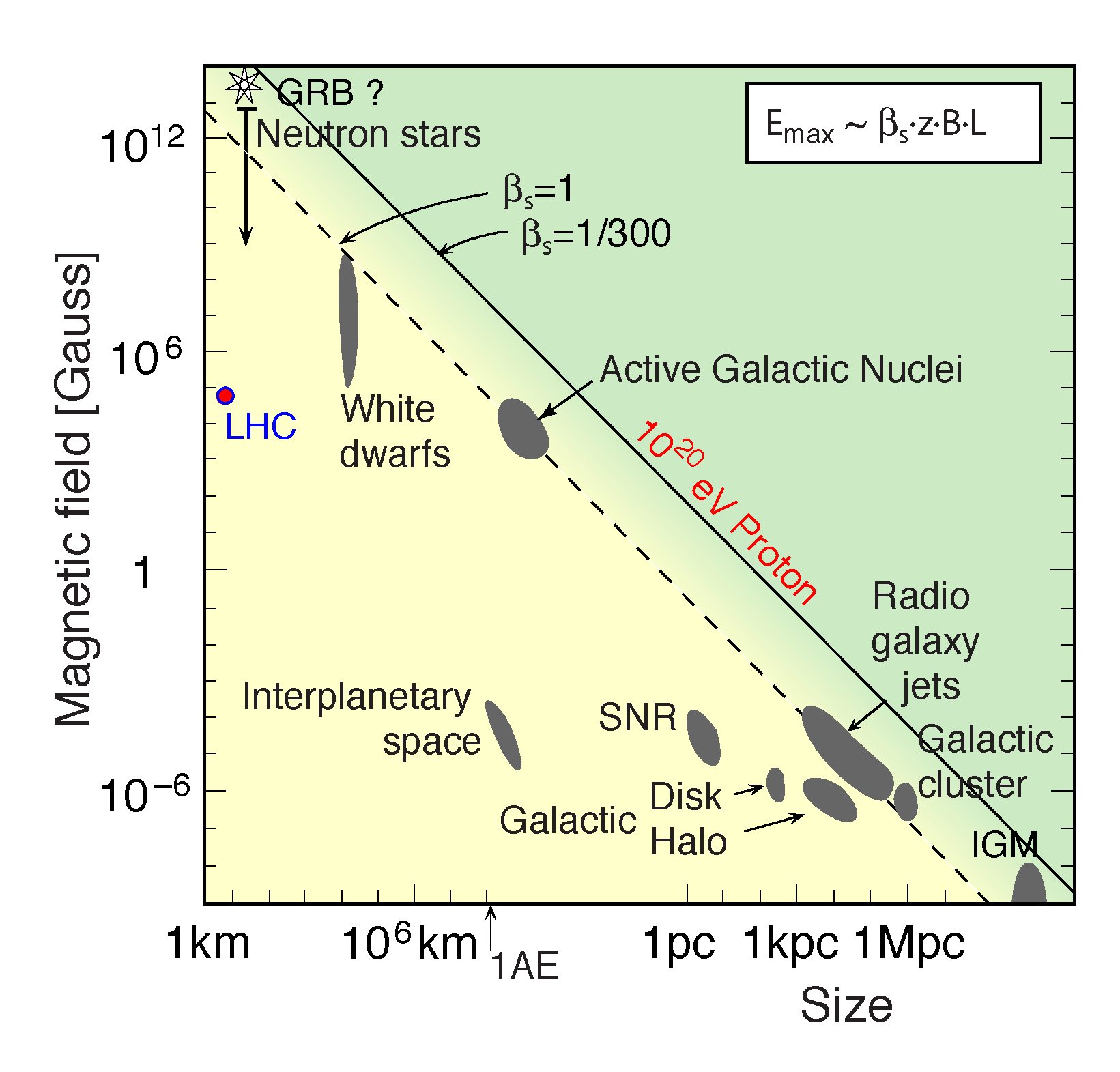
Hillas Criteria
The equation of the maximum energy from shock acceleration can be rewritten as:
\[E_{max} \leq 10^{18} \mathrm{eV}\; Z \;\beta_s \left(\frac{R}{\mathrm{kpc}}\right)\left(\frac{B}{\mu\mathrm{G}}\right)\]
where \(\beta_s\) is the shock velocity, \(B\) the magnetic field strength, and \(R = u_1 t_{age}\) is the radius of the expanding shockwave, or in other words the size of the acceleration reguin. In 1984 Hillas arrived to a similar conclusion just by doing a back-of-an-envelope assumption that in order for it to accelerate CR particles to high energies in which he impossed that a condition where the size of the acceleration region must be at least twice the Larmor radius. The plot showing possible sources in the parameter space \(B\) vs \(R\) is usually referred as the Hillas’ plot. For relativistic shockwaves (\(\beta_s \sim 1\)) many sources are able to accelerate protons up to \(10^{20}\) eV, however for slower shockwaves (\(\beta_s \sim 1/300\)) the number of source candidates is strongly reduced.
Sources of Galactic Cosmic Rays
Supernova Remnants (SNRs)
Supernova remnants (SNR) remain the most likely candidates for CR acceleration up to at least \(10^{14} \mathrm{ \; eV}\) via the Fermi shock mechanism. Supernova explosions are very violent events which transfer a significant amount of energy in the ISM. We distinguish between the SN explosions –the actual events and the next few years) and Supernova remnants - what happens over the next few thousand years. Supernova explosion mechanism can be the carbon deflagration of white dwarts (Type I) or the core collapse of masssive stars (Type II) but the dynamical evolution of the supernova remnant (SNR) i.e., the expanding cloud of hot gas in the ISM is similar and can be divided in 3 phases depending on the relation between the ejected material, \(M_{ej}\) and the swetp material \(M_{sw}\):
Free Expansion Phase.\(M_{ej} \gg M_{sw}\) The shock wave moves in the ISM gas a highly supersonic speed. The speed is constant as there is no acceleration and so the shock radius scales as \(R_s(t) = v_e t\). Behind the shockfront ISM gas starts to accumulate an a reverse shock starts to form. Sometimes we see first this reverse shock. At some point the compressed ISM gas equals the ejected material, this marks the end of the free expansion phase. Given an initial density of ISM \(\rho_{ISM}\) we can can define a swept material as: \[M_{sw} = \frac{4\pi}{3}\pi R_{sw}^3\rho_{ISM}\] When the condition \(M_{sw} \simeq M_{ej}\) is reached, this marks the end of the free expansion phase and the swept radius can be defined as: \[R_{sw} = \left(\frac{3M_{ej}}{4\pi\rho_{ISM}}\right)^{1/3}\] This radius is reached at the defined swept time \(t_{sw} =R_{sw}/v_{sh}\) which is about 200-300 years.
Sedov-Taylor Phase. Once the reverse shock reaches the nucleus, the interior of the SNR gets very hot that energy losses due to radiation are not possible (all atoms are ionized). The cooling of the gas is only due to the expansion, that’s why this phase is the adiabatic phase. This is therefore a pressure-driven phase. Taking the pressure into account we can use the following formula: \[\frac{\textrm{d}}{\textrm{d}t}(m v) = F\]\[\frac{\textrm{d}}{\textrm{d}t}\left(\frac{4\pi}{3}R_{sh}^3\rho_{ISM}\dot{R}_{sh}\right) = 4\pi R^2_{sh}P\] The pressure and internal energy \(E\) of an ideal gas are related by: \[P = (\gamma -1)\frac{E}{V}\] where \(V\) is the volume. Since this is an adiabatic expansion we can assume that the internal energy is equal to the explosion energy \(E =E_{SN}\), and \(V = 4\pi R_{sh}^3 /3\). Assuming a mono-atomic gass with a adiabactic index \(\gamma = 5/3\) we obtain as pressure: \[P = \frac{E_{SN}}{2\pi R_{sh}^3},\] which inserting on the expression above we have:
\[\frac{\textrm{d}}{\textrm{d}t}\left(\frac{1}{3}R_{sh}^3\rho_{ISM}\dot{R}_{sh}\right) = \frac{E_{SN}}{2\pi R_{sh}}.\] Solving for \(R_{sh}\), assuming it has a form of \(R_{sh} \propto t^\eta\) we obtain: \[R_{sh}(t) = \left(\frac{25E_{SN}}{4\pi \rho_{ISM}}\right)^{1/5}t^{2/5}\]\[v_{sh}(t) = \frac{2}{5}\left(\frac{25E_{SN}}{4\pi \rho_{ISM}}\right)^{1/5}t^{-3/5}.\]
As can be seen, the radius goes as \(R_{sh} \propto t^{2/5}\). When temperature reaches the critical value of \(10^{6}\) K ionized atoms start to capture free electrons and can lose energy due to de-exitation. This is the end of the adiabatic phase. This phase can last 20,000 years.
Cooling or Snowplough phase Due to the effective radiative cooling the thermal presure decreases and the expansion slows down. More and more interstellar gas is accumulated until the swept-up mass is much larger than the ejected material. Finally the shell breaks up into clumps probably due to Rayleigh-Taylor inestabilities. This phase lasts up to 500,000 years.
As we discussed, the \(E_{max}\) depends on how long the accelerator is active. Therefore an individual CR particle will gain the highest energy if it starts during the free expansion phase and stays within the shock front until and through the Sedov phase. There is a caveat though, the \(E_{max}\) also depends on the magnetic field, and magnetic fields during the slow expansion of the Sedov phase are not strong enough to confine the CR particle. In this case, it seems the maximum CR energy may only be reached during the pre-Sedov expansion. This is the reason why young SNR are the main candidates to search for CR injection up to PeV energies.
Other Sources of Galactic Cosmic Rays
Neutron stars
A neutron star is a stellar remmant that results from the collapse of a massive star after a supernova. As the core of a massive star is compressed during the supernova, the reaction \(e^- + p \rightarrow n + \nu_e\) can take place which transforms the core into a neutron rich matter. Neutron stars, especially young fast-rotating pulsars and magnetars have extreme magnetic fields (up to \(10^{12}\; \mathrm{G}\) in the case of magnetars) with complex structure that could accelerate CR up to the highest energies. These objects are far rarer than SNRs, however, only a dozen magnetars are known in the Milky Way, although many could exist in the local neighborhood.
Microquasars
Microquasars are radio-intense X-ray binary stars with a companion orbiting an accreting compact object. They are particularly interesting particle accelerators due to observation of VHE gamma ray emission and highly relativistic jets which could provide energy for UHECR