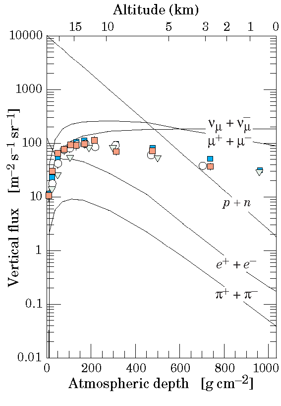
The plot below shows the particle flux surviving after a certain altitude.
Source: Particle Data Group
We can extract different information from this plot:
Primaries dominate up to 9 km, secondaries (electrons, pions) roughly follow the primary shape. Muons and neutrinos are continously produced.
Vertical fluxes for \(E > 1\) GeV. Points show the \(\mu^-\) measurements. Muons and neutrinos are produced in decays of mesons which are themselves produced by interactions of CR particles with air nuclei.
They are the dominant flux at sea level and the only ones that can penetrate deep underground.
Electrons and nucleons fluxes above 1 GeV/\(c\) are about 0.2 and 2 m\(^{-2}\) s\(^{-1}\) sr\(^{-1}\) at sea level. Nucleons are the degraded remnants of the primary cosmic radiation. At sea level about 1/3 are neutrons.
Muons and Neutrinos Production
The most important channels for muon and neutrino production are:
For each of the 2-body decay channels, assuming the muon always decay the neutrino flavor ratio is:
\[\mathbf{ \nu_\mu : \nu_e = 2:1}\]
Mean free path for mesons, \(\pi\), \(K\)
Charged pions and Kaons can interact or decay. Both processes have a mean free path and one or the other will dominate depending on which mean free path is larger.
The decay mean free path of pions is given by \(l^d_\pi =\gamma c \tau_\pi\) where \(\gamma\) is the Lorentz factor of the pion. Multiplying for density we have the density decay mean free path as:
\[\lambda^d_\pi = \rho(X) \gamma c \tau_\pi\]
However the atmosphere density depends on the atmospheric depth as \(\rho(X) = X/h_0\). In units of slant depth, \(X_{sd} = X/\cos\theta\) and expanding \(\gamma = E / m_\pi c^2\) we can rewrite the density decay free path as:
as a critial energy. The crital energy is such that the decay time equals the vertical atmospheric depth \(\lambda^d_\pi(\epsilon_\pi) = X_{sd} \cos\theta = X\).
The interaction mean free path is the same as nucleon \(\lambda_\pi = A m_\pi/\sigma_\pi^{air}\) which as we saw is indenpendent of \(X\).
Critical energy for mesons, \(\pi\), \(K\)
Decay or interaction dominates depending on whether \(1/\lambda^d_\pi\) or \(1/\lambda_\pi\) is larger. This in turns depends on the ratio between the energy \(E\) and the critical energy \(\epsilon_\pi\). For example, the value of the crital energy for pions is given by:
For \(E \gg \epsilon_\pi\) decay length is much larger than the atmospheric depth, so interaction dominates.
For \(E \ll \epsilon_\pi\) decay dominates is much shorter than the atmospheric depth, so the pion will likely decay before interacting.
The same formulas can be derived for Kaons.
Muon Fluxes
The muon energy spectrum at sea level is a direct consequence of the meson source spectrum. Unlike electrons, muons will decay before reaching the ground in the GeV energy range. The muon decay length is given by:
\[ d_\mu = \gamma \tau_\mu c\]
Where \(\tau_\mu\) is the muon lifetime of the order of \(2.2\times 10^{-6}\) s. So for a muon of 1 GeV we have:
lifetime =2.1969811e-6# muon lifetime in secondsimport scipy.constants as ctecspeed = cte.cmuon_mass = cte.value("muon mass energy equivalent in MeV") *1e-3# in GeVenergy =1# GeVprint(f"d = {(energy/muon_mass)*lifetime*cspeed*1e-3:.2f} km")
d = 6.23 km
Compared to the typical atmospheric altitude of \(h \sim 15\) km it means that at those energies, muons will not reach the ground.
Energy Regimes of Muon Fluxes
Three different regimes are distinguishable:
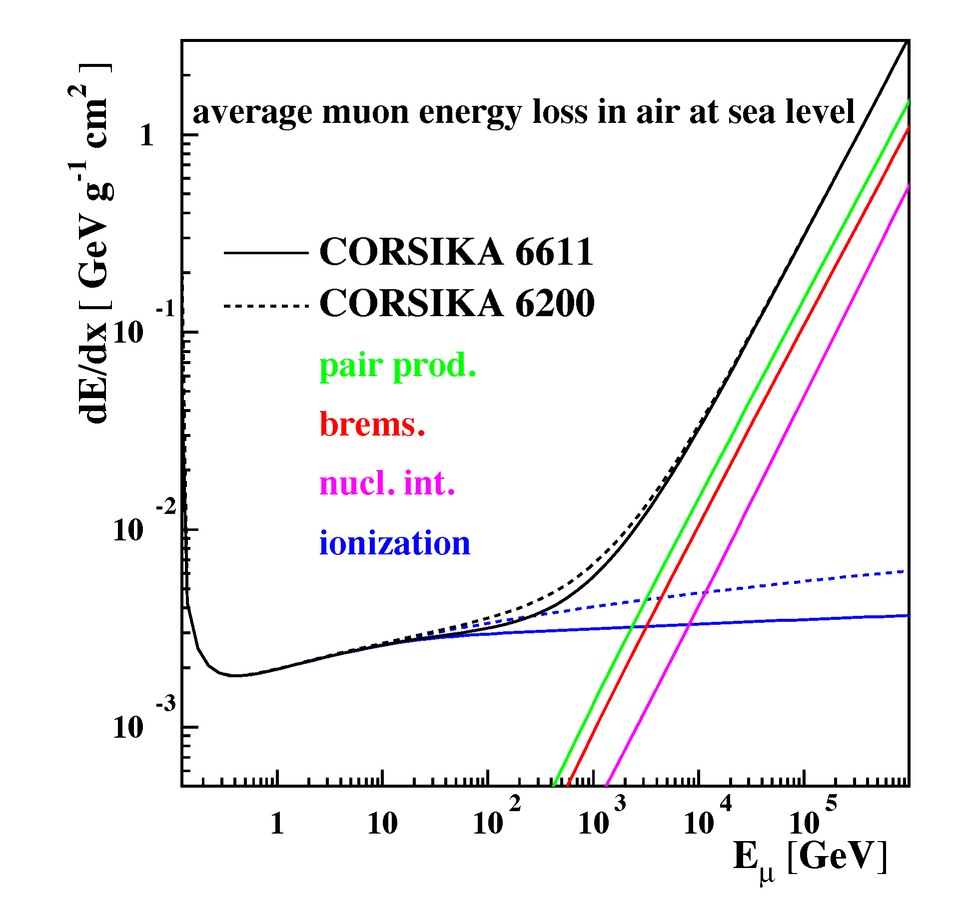
\(E_\mu \leq \epsilon_\mu\), where \(\epsilon_\mu \sim 1\) GeV. This critical energy is when interaction probability and decay probability start to be comparable. Even more the muon energy losses become important. As we saw energy losses via ionization is almost constant, for muons is about \(\sim 2\) MeV/(g/cm\(^{2}\)) in air (and mostly independent on the material). However this is true only above energies of 1 GeV, below ionization losses increase drastically as can be seen in the figure below.
\(\epsilon_\mu \leq E_\mu \leq \epsilon_{\pi,K}\), where \(\epsilon_\pi = 115 \;\mathrm{GeV}\) and \(\epsilon_K = 850 \;\mathrm{GeV}\). In this range all mesons decay and muons spectrum follows the same of the parent spectrum of mesons and hence that of the primary CRs. The muon is almost independent of the zenith angle.
\(E_\mu \gg \epsilon_{\pi,K}\), Mesons interaction length starts to be comparable to their decay length. This happens first for inclined showers and so the muon flux gets suppressed while it also starts to depend on the zenith angle (ie on the density of the atmosphere).
At even highers energies, above 1 TeV in air, muons will also start to loose energie via other radiative process (we will see that below when talking about muons underground).
Muon Flux Analytical Approximation
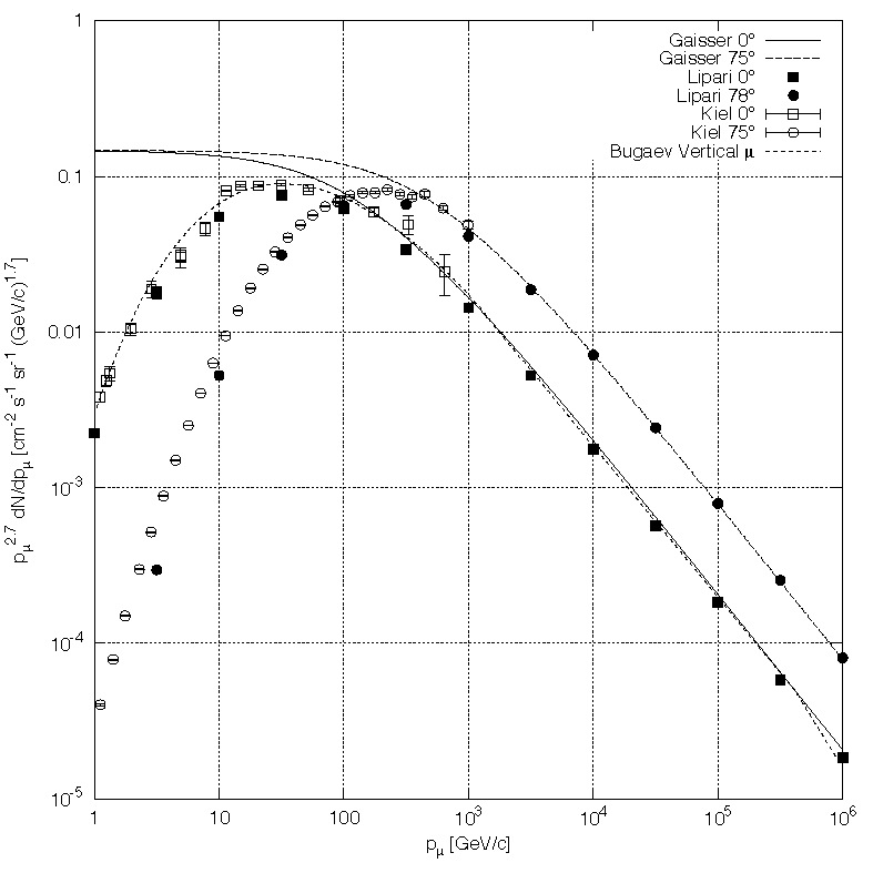
An approximate extrapolation formula valid when muon decay is negligible (\(E_\mu > 100/\cos\theta\) GeV) and the curvature of the Earth can be neglected (\(\theta < 70^{\circ}\)) is given by the Gaisser parametrization:
In reality below 10 GeV muon decay and energy loss become important and the Gaisser parametrization overestimates the muon flux as can be seen in the plot below:
Source: Particle Data Group
As can be seen from the measured muon flux has the following characteristics:
Muons are the most numerous charged particles at sea level
The mean energy of muons at the ground is \(\sim\) 4 GeV.
The integral intensity of vertical muons above 1 GeV/c at sea level is \(\approx 70 \mathrm{m}^{-2} \mathrm{s}^{-1} \mathrm{sr}^{-1}\) or \(\approx 1 \mathrm{cm}^{-2} \mathrm{min}^{-1}\).
Muon Bundles
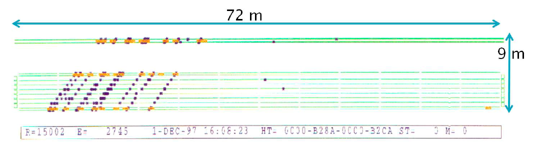
Sometimes muons also come in groups or bundles of parallel muons originated from the same primary CR. Muon bundles sometime look like a single high energy muon. The multiplicity (number of muons in the bundle) if can be measured is correlated with the mass of the orignal CR. The image belowe shows a muon-bundle event observed with the MACRO underground detector.
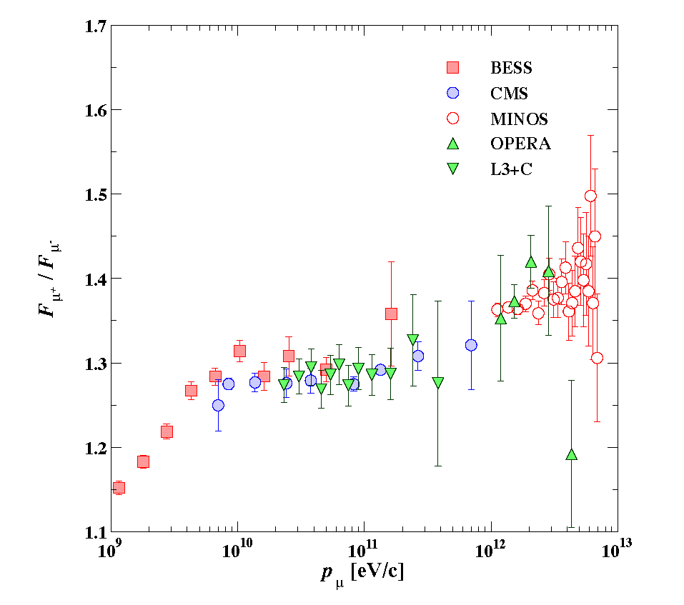
Muon anti-Muon Charge Ratio
The muon charge ratio reflects the excess of \(\pi^+\) over \(\pi^-\) and \(K^+\) over \(K^-\) and the fact that there are more protons than neutrons in the primary spectrum.
Neutrinos are the most abundant CR product at sea level, yet they have only recently (compared to other particles) measured due to their extremely low cross-section.
The process giving neutrino fluxes are the same as for the muons (we saw already) plus the muon decay. Taking into account the decay of pions, kaons and muons gives to a flavor ratio of: \(\nu_\mu : \nu_e = 2:1\) and \(\nu_e/{\bar \nu_e} \sim \mu^+/\mu^-\)
At few GeV (> \(\epsilon_\mu\)) muons will not decay and \(\nu_e\) will be supressed as the main source of \(\nu_e\) is the muon decay.
Tutorial II: Plot the \(\nu_\mu\) and \(\nu_e\) atmospheric flux using the package DaemonFluxYañez and Fedynitch (2023)
As mentioned neutrinos and muons are strongly correlated. However due the two-body kinematics, the energy spectra of the \(\nu\)’s and \(\mu\)’s from mesons decay are different. For example, the energy of the muon in CoM is given by:
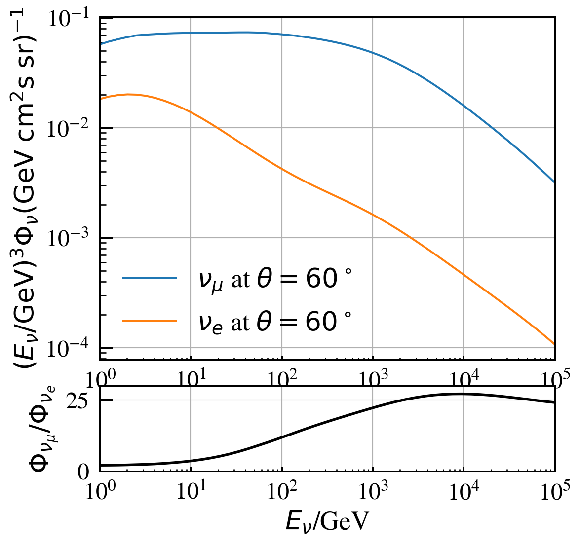
In the laboratory system, the energies are boosted by the Lorentz factor \(\gamma= E_\pi /m_\pi\), but as can be seen muon carry a much larger fraction of energy than neutrinos. For energies about \(1\;\mathrm{TeV}< E_\nu < 10^3\;\mathrm{TeV}\), the angle averaged atmospheric \(\nu_\mu + {\bar \nu_\mu}\) can be approximated by a power law spectrum:
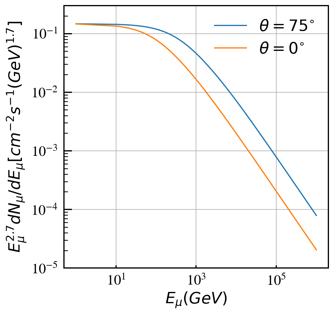
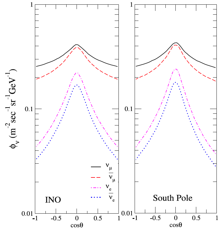
Another difference with respect to the muon fluxes is their dependency with respect to the zenith angle. Since atmospheric muons are not absorved by the Earth, their spectrum spans to the whole sky. The following plot shows the calculated neutrino flux at 1,300 m depth with energies \(E_\nu = 10\) GeV.
The peak at the horizon in the atmospheric neutrino flux is due to the so-called secant theta effect. This effect occurs because pions and kaons that are produced nearly skimming the Earth have more flight time in less dense atmosphere, so they have more chance to decay than interact.
Prompt Fluxes
Apart from kaons and pions, charmed messons will also be produced in the atmosphere. Charm particles have lifetimes so short (\(10^{-12}\)s) they almost alway decay before interacting. Muons and neutrinos from charm decay are called prompt muons/neutrinos. They have the following peculiarities:
The energy spectrum follows the one of the primary cosmic rays ie that of \(\sim E^{-2.7}\).
Since there is no competition between decay and interaction of the charm particle, the prompt flux is fully isotropic.
Since neutrinos are produced in 3-body decays they produced the same amount of \(\nu_\mu\) and \(\nu_e\).
It is important to note that the prompt fluxes have not been observed yet.
Yañez, Juan Pablo, and Anatoli Fedynitch. 2023. “daemonflux: DAta-drivEn MuOn-calibrated Neutrino Flux,” February. https://arxiv.org/abs/2303.00022.